In recent years, scientific tools have been increasingly applied to the study of artwork, for numerous reasons: determination of authenticity, determination of provenance, analysis for restoration, or even for finding ‘hidden’ art buried behind or underneath existing masterworks.  Some time ago, Jennifer at Cocktail Party Physics wrote a fascinating post on the use of X-ray imaging for the latter application.

Around that same time, an entire issue of Applied Physics A was devoted to the “Science and Technology of Cultural Heritage Materials: Art Conservation and Restoration.”  The first paper in the issue is an overview of “Optical coherence tomography in art diagnostics and restoration,” by P. Targowski, B. Rouba, M. Góra, L. Tymińska-Widmer, J. Marczak and A. Kowalczyk.  Though it has been a few months since the paper’s release, I wanted to write a bit about optical coherence tomography and how it is being used in the analysis of artwork.

So what is optical coherence tomography? It is an optical interferometric technique for imaging the subsurface structure of scattering materials.  It was initially developed in the late 1980s as a medical diagnostic tool and was applied to measurements of the human eye, but since that time it has exploded into a technique widely used for numerous applications, both in the medical field and outside of it.  In medicine, OCT has been used for studies of cardiovascular problems (heart disease, stroke), musculoskeletal problems (osteoarthritis), as well as in oncology (cancer detection).

Curiously, I’ve had a difficult time finding a clear explanation of the physics of OCT.  If I were to speculate, I would say there are three reasons for this:  1.  It is a technique developed and propagated by medical professionals who are far more interested in application than explanation, 2.  There are now countless different techniques labeled as ‘OCT’, each of which works in a significantly different way, and 3.  The technique relies on the theory of optical coherence, which is not widely understood anyway!  I will introduce the technique by first looking at the related technique of ultrashort pulse optical rangefinding, and work my way through the two major types of OCT, time-domain OCT and frequency-domain OCT.

Let us first imagine that we have a one-dimensional multilayered system whose structure we wish to map out in detail.  For simplicity, we imagine that the system consists of a collection of partially reflective sheets of material, and we are allowed to perform optical measurements only from the ‘outside’ of the system, at the plane :

A rough technique to measure the positions of the different planes is to send a very short pulse of light into the system.  By measuring the ‘time-of-flight’ of the pulse, i.e. how much time passes before the ‘echoes’ of the pulse return to the source/detector, one can estimate the location of each of the planes.  The structure above, for instance, might produce the following response:

Knowing that the speed of the light signal is , the round trip time of the pulse from the plane at location is simply .   From this echo recording we can produce a rough picture of the structure.  This is the same principle that is used by radar systems to determine target distance.

This technique is extremely simple in principle but costly in practice, as the resolution of the image is dependent upon the width of the pulse: objects which are closer together than the width of the pulse cannot be distinguished.  This is illustrated below for the same system as above, but with a wider illuminating pulse:

In this case, the echo pulses from each of the planes will overlap.  In the overlap area, they will produce interference fringes which will further confuse the interpretation of the data.  To achieve a resolution on the order of a micron ( meters), one must use a pulse of that length, which translates into a pulse of duration

,

or a femtosecond-length pulse!  This is certainly possible, but femtosecond lasers are relatively complex, expensive systems, which limits their broad application in medicine.

A simpler and cheaper alternative is to use a source of light with extremely low temporal coherence, and use the interference properties of the ‘echo’ signal to determine distance.  This is done with our old friend the Michelson interferometer (I discuss its application here and here), illustrated below:

The Michelson interferometer takes as an input a beam of light from a source , which is divided into two components at a beamsplitter .  Each component is reflected from a mirror, returning it to the beamsplitter.  The beamsplitter recombines the two light signals and projects the result onto a screen .  The light passing along leg 1 of the interferometer travels a distance farther than the light passing along leg 2.  As discussed in the ‘optics basics’ post on coherence, the two beams will only produce an interference pattern if this distance is less than the coherence length of the light field, i.e.

for interference.  One application of this interferometer is to measure the coherence length of the illuminating light field, by measuring the distance over which the system produces interference.  If is very small, however, there will only be interference when .  This suggests another use of the interferometer: with low coherence light sources, we can use interference to measure distances in our sample.

This is the basis of time-domain OCT, and is illustrated schematically below.

When the reference mirror is positioned at a distance coincident with one of the layers of the sample, interference fringes will become visible.  This system maps out the position of the layers via fringe visibility just as the time-of-flight measurement maps them out via the time delay of the return pulses.

The technique we have described so far is only used to map one-dimensional layered structures.  A full two- or three-dimensional image of a sample can be mapped out by scanning the incident field, or a probe emitting the incident field, transversely across the surface of the sample.  An OCT image of the macula, taken from www.eyetumour.com, is shown below:

The term ‘optical coherence tomography’ was apparently first coined in 1991* in a Science paper by D. Huang et al., though this sort of low coherence interferometry goes back at least as far as 1988, when A.F. Fercher et al. made in vivo measurements of the length of the human eye**.  As we have noted in a previous post, the word ‘tomography’ is derived from the Greek tomos (slice) and graphein (to write). It is not clear to me what ‘slice’ is being measured in this technique; it seems that the term ‘tomography’ in this case is being used as a synonym for ‘computational imaging.’

The original OCT system by Huang et al. used a superluminescent diode (of center wavelength 830 nm) as a source of low-coherence light.  A longitudinal resolution of 17 microns was achieved.  Because human tissue is not particularly transparent to visible light, the scans were limited to a distance of at most 1 to 2 milimeters in depth.  For in vivo studies of deep-seated tissues, a catheter can be used to get the probe to the target.

Though the ‘time-of-flight’ and  OCT seem like very different techniques, they are in fact mathematically very closely related.  A pulse of duration and its spectral width are constrained by the Fourier uncertainty relation,

.

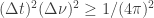
This inequality is entirely due to the wave properties of the pulse; in quantum mechanics, the wave nature of matter gives rise to the mathematically similar Heisenberg uncertainty relations.  The consequence of this inequality is that a narrow pulse tends to have a broad spectrum, and vice versa, as illustrated below:

A function with a broad temporal profile will have a very narrow spectral profile , and vice versa.

For a low-coherence CW (continuous wave) field, an identical relationship holds between the coherence time and the spectral width of the field,

.

A CW field with a small coherence time will have a broad spectrum, and vice versa.  Both optical pulses and partially coherent CW fields can be represented as a combination of a collection of monochromatic (single-frequency) fields, using the mathematical methods of Fourier analysis.  The only difference between a pulse and a partially coherent CW field is that, for a pulse, the monochromatic components have a definite phase relationship to each other, while in a PC CW field, the monochromatic components have no definite phase relation.

Both ‘time-of-flight’ measurements and TD-OCT measurements therefore require a probing field which contains as many frequencies of light as possible, apparently the more the better.  This suggests that each frequency of light used in probing the sample contains unique information about the object’s structure.  This observation is the basis of the more recent technique of spectral OCT***, in which the interference pattern produced by partially coherent light reflecting from the sample is analyzed frequency-by-frequency.  The advantage of such a system is that there is no longer any need to scan the position of the reference mirror, and it runs much faster than a TD-OCT system.  In short, the original TD-OCT system was inefficient in that it could not measure and therefore ‘wasted’ information about the relative contributions of the different frequencies to the interference pattern.

We now return to the use of OCT in art diagnostics and restoration!  The work is being done at the Institute of Physics at Nicolaus Copernicus University in Poland, in the medical physics group.  S-OCT is used to measure the thickness of layers of paint and varnish in oil paintings, with an emphasis on studies of the artist’s signature.  There are a number of reasons to do this, broadly grouped into issues of provenance and restoration.  Traditionally, analysis of the layers of a painting would require the removal of a sample from the painting, a step one would like to avoid for obvious reasons.

Concerning the issue of provenance, the review article focuses primarily on forgeries: apparently a common method of faking signatures on older artwork is to paint it upon the original varnish and then cover it with an extra layer of lacquer.  Without an examination of the layers, it is difficult if not impossible to distinguish between this ‘varnish-signature’ and a signature in the original paint.  As the signature is one of the most important areas of a painting, it is impractical to damage it by extracting physical samples.  An OCT scan, however, is non-invasive and can determine whether the signature is present in the original paint or an upper varnish layer.  The Polish researchers tested this with a 20th century painting done in the style of a 17th century Dutch master, and were clearly able to identify a ‘varnish-signature’.

Anyone who has been to an art museum is also painfully aware that varnish can obscure legitimate details in artwork.  The research group also demonstrated the ability to retrieve depth information of a legitimate signature buried in varnish which was otherwise almost unreadable to the naked eye.

In art restoration, it is often desirable to remove the varnish layer to make the underlying paint accessible to ‘touching up’.  Laser ablation — basically blasting the varnish off with a laser beam — is a standard method for doing so.  Obviously, one does not want to remove any paint in the process.  The standard technique to avoid this is to use Laser Induced Breakdown Spectroscopy: when the paint begins to be evaporated, it generates a plasma whose spectral signature can be detected.  This still involves paint removal, however, and is an ineffective technique if one wishes to only partially remove the varnish from a location.  OCT seems to be a viable alternative for measuring the amount of ablation from the paint surface, and the Polish group were able to dynamically measure the ablation process with a recording rate of 15 frames/s.  The researchers demonstrated that the ablation process differs for different types of varnish.  Some varnishes directly evaporate, while others melt.  A better understanding of these processes will obviously improve the effectiveness and safety of ablation processes.

The researchers extended their OCT studies beyond painting and into the realm of stained glass.  It is almost impossible to remove layered samples from glass without damage, and traditionally examinations have been restricted to studying the edges of sheets which have been taken from their frames.  The Polish group was able to demonstrate non-destructive imaging of a section of stained glass.

When I first heard of OCT years ago, it sounded too simple to be true: the one-dimensional scans ignore transverse scattering, and basic OCT calculations ignore the phenomenon of dispersion (which would distort the image). This shows a big limitation of being a theorist: I couldn’t justify ignoring such complications from a theoretical point of view, but the experimentalists just went out and showed that the experiments worked!  OCT has become an important imaging technique in medicine and, as the research described here shows, it has found even more uses in the art world.

Thanks to stuwat for suggesting and helping inspire this post!

********************

* D. Huang, E.A. Swanson, C.P. Lin, J.S. Schuman, W.G. Stinson, W. Chang, M.R. Hee, T. Flotte, K. Gregory, C.A. Puliafito, J.G. Fujimoto, “Optical coherence tomography,” Science 254 (1991), 1178.

** A.F. Fercher, K. Mengedoht and W. Werner, “Eye-length measurement by interferometry with partially coherent light,” Opt. Lett. 13 (1988), 186.

*** See A.F. Fercher, C.K. Hitzenberger, G. Kamp and S.Y. El-Zaiat, “Measurements of intraocular distances by backscattering spectral interferometery,” Opt. Commun. 117 (1995), 43, and S.R. Chinn, E.A. Swanson and J.G. Fujimoto, “Optical coherence tomography using a frequency-tunable optical source,” Opt. Lett. 22 (1997).

P. Targowski, B. Rouba, M. Góra, L. Tymińska-Widmer, J. Marczak, A. Kowalczyk (2008). Optical coherence tomography in art diagnostics and restoration Applied Physics A, 92 (1), 1-9 DOI: 10.1007/s00339-008-4446-x