
One of the tragedies of STEM education is the seemingly eternal perception by the general public that mathematics is boring and repetitive. Most people, of course, end their math education with algebra at most, though some work their way through a calculus course before leaving for good.
This is a tragedy because mathematics is one of the best fields to find incredibly beautiful objects, experience mind-blowing concepts that challenge ones imagination — or sometimes both simultaneously.
A wonderful example of this is the geometric object constructed by the Italian mathematician Giuseppe Peano and described in his 1890 paper “Sur une courbe, qui remplit route une aire plane.” This beautiful and mind-boggling object is illustrated below.

Uh… wait a minute…
*shuffling of papers as I check my notes*
No, that is correct! The object above is obviously a square, which at first glance would seem to be the most boring geometric figure possible. What Peano did, however, was demonstrate a new way to fill the square, inventing a mathematical construction that allows the square to be completely filled in with a single, continuous line! This “Peano curve” was the first example of what is now known as a space-filling curve, which has surprising and insightful connections to modern mathematics.
Giuseppe Peano (1858-1932) was a brilliant and creative mathematician who had a major influence on a number of fields of mathematics, including set theory, logic, and axiomatic mathematics. We have recently come across his work on this blog in the context of the science of falling cats, which inspired Peano to dabble in the physics of the Earth’s motion — though his geophysics research was not particularly groundbreaking*.
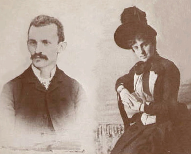
Giuseppe Peano and wife Carola Crosio in 1887, via Wikipedia.
In the early 1890s, however, Peano had come across the stunningly novel work of Georg Cantor on set theory, in particular the description of the different sizes of infinity. We have discussed this in a series of posts on this blog before**: in short, Cantor noted that the set of real numbers between 0 and 1, dubbed the continuum, is an infinitely larger set than the set of counting (natural) numbers 1,2,3,… . The “size” of the continuum is labeled 

This was a difficult enough concept for many to accept; even stranger, Cantor proved that the size of the continuum — the set of points between 0 and 1 — is just as large as the set of all point in a square! That is, if one considers every distinct point on the number line, they can be lined up in a one-to-one correspondence with every distinct point in a square.
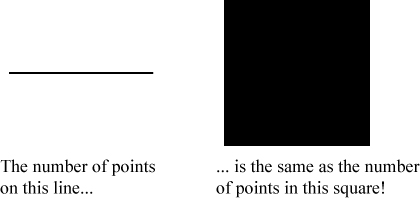
This is, obviously, a very non-intuitive result! We know that a square is a two-dimensional object, while a line is a one-dimensional object; it does not seem that a line could contain the same number of points. Nevertheless, Cantor demonstrated that this is true, using very simple logic (described in my infinity post series, part II).
In the wake of Cantor’s revelation, however, another question arose: is it possible to continuously map a line into a square? In other words: is it possible to draw (mathematically, at least) a single continuous curve that fills a square entirely? To be continuous, the square must be filled by a mathematical pen that is never lifted from the mathematical paper, kind of like a “connect the dots” kids puzzle whose outcome is a filled black square.

A partially filled “connect the dots,” via Wikipedia.
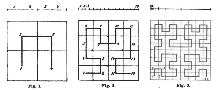
Peano was the first one to introduce such a curve, now known as a space-filling curve. As one might expect, such a curve is quite unusual, and won’t quite look like anything encountered before. In fact, the complete curve is impossible to visualize, since it literally fills the square and, in the process, takes an infinite number of twists and turns along the way. However, we can get a feel for its behavior through an iterative process that generates curves of increasing complexity that approach the true space-filling curve in the limit of infinite iterations. The result of the first four iterations of the Peano curve are shown below.
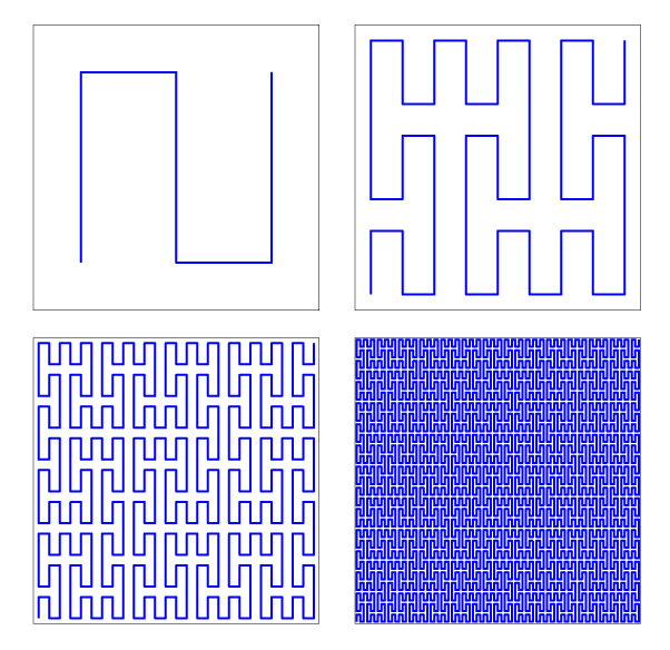
The starting point of the Peano curve is basically a sideways, backwards “S.” In the next iteration, that basic “S” is preserved — the path meanders up, then down, then up again — but takes additional detours along the way. In the next iteration, detours of detours are taken, and so on. Even by the fourth iteration, one can see that the curve is starting to fill in the entire square; with an infinite number of iterations, it completely fills it in.
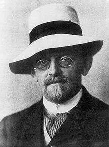
David Hilbert (1862-1943), mathematical badass. Via Wikipedia.
Curiously enough, the first person to give a graphical representation of a space-filling curve was not Peano, but the great German mathematician David Hilbert. Peano’s paper (an English translation by me can be found at this link) gives a detailed mathematical description of the curve, and a proof that it does in fact completely fill a square, but does not give any illustrations. Curiously, Peano apparently knew how to do so, as it is reported that he installed a tiled representation of the curve on the terrace of a villa he purchased in 1891***. On reading Peano’s paper, though, Hilbert immediately realized that one could generate the curve by an iterative procedure such as pictured above.
Hilbert demonstrated the process by creating a new, (relatively) simpler space-filling curve, which he published in an 1891 paper, “Ueber die stetige Abbildung einer Linie auf ein Flächenstück.” Hilbert’s original drawing of the creation of the curve is shown below.
These pictures give a simple idea of how the process works. Hilbert noted that, in his curve, the line could be divided into four segments, and each segment of the line corresponds to 1/4 of the entire square. Then, each of the four line segments can be divided into four smaller segments, and each of those segments corresponds to 1/4 of each of the smaller squares, and so on. This process results in an increasingly convoluted path with each iteration.
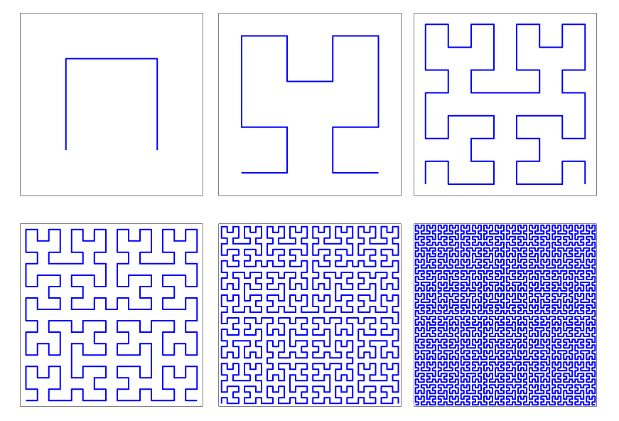
Using my own code, the first 6 iterations of Hilbert’s curve are shown below.
The key to generating the Hilbert curve is to notice that the structure looks similar, albeit smaller, at each level. In fact, the 2nd form of the Hilbert curve above consists of four shrunken copies of the original curve, appropriately joined together. Step 1 is shown below.
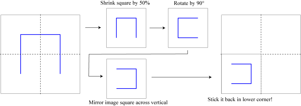
Step 2 is simply shrinking the original square and moving it to the upper left corner.
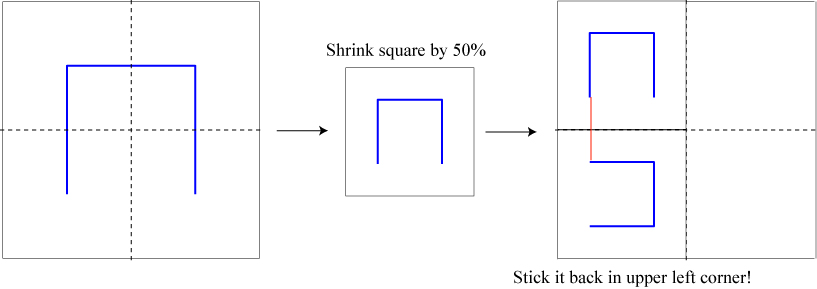
Note the red line that has been added to connect the two pieces! The third step involves shrinking the original square and moving it to the upper right corner.
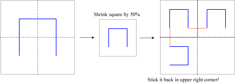
Finally, we perform a final series of transformations to get the final piece.
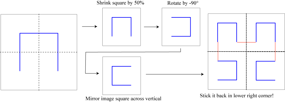
We have the next iteration of the Hilbert curve! To get the next iteration, we take this current iteration and perform the same four operations on it, and so on, and so on! A Peano curve is generated in a similar manner, the main difference being that the square is divided into nine pieces, and each iteration produces nine shrunken, rotated and mirrored copies of the previous iteration.
This process, however, indicates that a Hilbert curve and, similarly, a Peano curve, have the same structure on different size scales. In other words: if you zoom in on a part of the curve closer and closer, it looks pretty much the same. For some readers out there, this will sound suspiciously familiar: it sounds like a fractal!
For those unfamiliar, a fractal may be loosely defined as a geometrical object that is self-similar at different zoom levels. The concept was introduced by Polish mathematician Benoit Mandelbrot in the 1970s, and it can describe many real-world objects that look similar near and far away: clouds, coastlines, mountaintops.
A classic and very familiar example of a fractal is a Sierpinski triangle, as shown below.

A classic Sierpinski triangle.
This triangle can be created in a number of different ways, but one way is directly connected to the space-filling curve construction. Start with a full triangle (or a single point) in the middle of the unit square. Shrink this triangle or point in half, and move three shrunken copies to the corners of the original triangle. Keep doing this process, and the Sierpinski triangle forms.
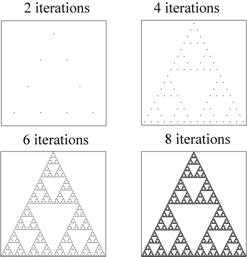
Development of the Sierpinski triangle.
One of the most unusual properties of many fractal is that they possess a fractional dimension! For instance, although the Sierpinski triangle is spread out over the unit square, it is filled with “holes.” In a loose sense, it takes up more space than a traditional one-dimensional curve, but takes up less space than a traditional two-dimensional surface. In fact, it can be proven that the Sierpinski triangle has an effective fractional dimension of 1.585, between 1 and 2!
The space-filling curves of Hilbert and Peano may also be considered self-similar fractals. However, because they fill the entire square, their fractal dimension is simply 2! They are, in a sense, the weirdest sort of fractals because they are a complicated, self-similar structure that results in a very simple geometric object.
The choice of Sierpinski’s triangle to illustrate the relationship between fractals and space-filling curves is no accident: its “discoverer,” Wacław Franciszek Sierpiński (1882-1969), developed his own space-filling curve in 1912, after becoming obsessed with set theory a few years earlier. Wikipedia provides a charming summary of how this obsession began:
In 1907 Sierpiński first became interested in set theory when he came across a theorem which stated that points in the plane could be specified with a single coordinate. He wrote to Tadeusz Banachiewicz (then at Göttingen), asking how such a result was possible. He received the one-word reply ‘Cantor’. Sierpiński began to study set theory and, in 1909, he gave the first ever lecture course devoted entirely to the subject.
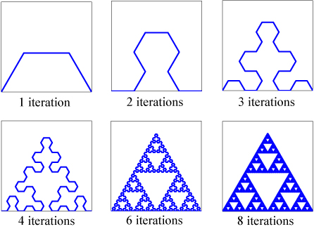
Sierpiński’s space-filling curve, not surprisingly, ends up filling a triangular region (though it can be adopted to fill a square quite readily). The first few iterations of this curve are shown below.

What about higher dimensions? Remarkably, Cantor not only demonstrated that it is possible to draw a curve that fills an area, it is also possible to draw a curve that fills a space of any number of dimensions. In three-dimensions, a Hilbert curve is readily constructed, as illustrated below.

Even more mind-boggling, it is possible to draw a curve that will fill a countably-infinite-dimensional region of space, i.e. a region of
There is at least one subtlety in the construction of space-filling curves worth noting. Even before Peano derived his curve, it had been shown by the German mathematician Eugen Netto (1848-1919) that it is not possible to draw a continuous curve that exactly fills the square. The implication of Netto’s theorem is that the Hilbert and Peano curves in fact over-cover the unit square: in the limit of infinite iterations, these space-filling curves run over themselves countless times.
So where does all of this information leave us? The work of Peano (and Cantor before him, and Sierpinski and Mandelbrot after him) demonstrates that the relationship between the dimensionality of an object and its structure is non necessarily a simple one. It is possible to construct a continuous “curve” that is one-dimensional, two-dimensional, fractional-dimensional, or infinite-dimensional. Peano’s work also demonstrates that beautiful mathematics can be found in even the simplest of squares!
P.S. The title of this post was inspired by this classic series.
Update: Interestingly, the Sierpinski triangle can also be constructed as a continuous line, known as the arrowhead curve. This is an explicit demonstration that a curve can be constructed that forms a structure with a fractional dimension.
********
For this post, I learned a lot about space-filling curves from the wonderful mathematical book by Hans Sagan, Space-Filling Curves (Springer Science & Business Media, New York, 1994).
********
* I’m so sorry for that.
** See part I, part II, part III, and part IV.
*** As described in Hubert Kennedy’s Life and Works of Giuseppe Peano (Springer, 1980).


remembering that all of this – countability, ordinal induction, pathological curves, dimension, content of a set, borel/lesbeque measure, clarification of interior/boundary/limit points, etc. all came from cantor figuring out if trig series representation of functions was unique, is pretty amazing
Well there was rather more to the motivation for topology and measure theory than just the question of sets of uniqueness for trig series.
Indeed! It is incredible how simple little questions can lead to huge revelations.
Fractal antennas are common. They interact identically with broad spectrum input.
http://classes.yale.edu/fractals/panorama/ManuFractals/FractalAntennas/FractalAntennas.html
http://www.fractenna.com/whats/whats.html
http://www.tsc.upc.es/fractalcoms/t11.htm
The link in the P.S. is obsolete, any other?
Replaced it. It’s a throwaway joke, anyway!