Another post inspired by my book on Falling Felines and Fundamental Physics! I talk about geometric phases in the book in the context of falling cats, but here I focus on the polarization of light.

I regularly argue that most physics isn’t as scary and complicated as most people think. Once you get past the mathematics, which is analogous to a foreign language for the non-fluent, many of the concepts and ideas are intuitive, and even logical. This is, in fact, the motivation behind all the physics posts on this blog!

But some concepts are resistant to easy explanation, and can be quite difficult to understand, even when you are familiar with all the math involved!  One topic that has vexed me, from an intuitive perspective, for a number of years is the concept of geometric phase.  Broadly recognized as a general phenomenon in physics due to the groundbreaking work of Michael Berry in the 1980s, the basic idea is as follows. Some physical systems can be brought from an initial condition, or “state,” changed through a variety of intermediate states and back into its original condition, yet nevertheless have something different about it.

The easiest example of this to visualize is Foucault’s pendulum, a free-hanging pendulum on the Earth, which I have discussed in detail before. Because the pendulum is oscillating on the Earth, and the Earth is effectively turning underneath it, the pendulum changes the direction of its swing during the day.

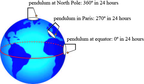
For a pendulum at the North Pole, the Earth spins 360º underneath it during a day, making the pendulum appear to change direction by 360º. A pendulum at the equator doesn’t change direction at all over the course of a day. But this means that a pendulum at some intermediate latitude, such as Paris, changes direction by less than 360º during the course of the day. Although the Earth has rotated back to its starting position, the pendulum has not ended up swinging in the same direction — that discrepancy is what we call the geometric phase.  It is “geometric” because its unusual behavior is related to the spherical geometry of the Earth.

So this case is somewhat easy to understand, but there is also a geometric phase associated with the behavior of light!  This phase, called the Pancharatnam phase for reasons which we explain below, is a bit trickier to explain. Recently, however, I found a very nice way to visualize this change, and how it connects to “geometry.” This is what I will (hopefully) show in this post!

Okay, before we dive into the “geometric phase of light,” we should talk about the nature of light, and what exactly we mean by the “phase” of light. It has been known since the early 1800s that light is a wave — that is, it is a disturbance that travels through a collection of variations in something, just like sound is a disturbance that travels through variations in the density of air pressure, and a water wave is a disturbance that travels through variations in the height of the water.  But what, in the case of light, is doing the “waving?” In the 1860s, Scottish physicist James Clerk Maxwell argued, correctly, that light is an electromagnetic wave: that is, the light that we see is in fact a combined electric field and magnetic field, oscillating together.  A simple illustration of this is shown below, with E representing the electric field and H representing the magnetic field.

So, if we had a detector that could measure the electric and magnetic fields as time passes, that detector would see those fields wiggling back and forth, swinging very much like a pendulum. (We cannot usually measure these individual wiggles, though, as visible light oscillates at a frequency of roughly a million-billion times per second.)

But these fields don’t just have to swing back and forth, or up and down. Again, much like the free-hanging Foucault pendulum, the field can swing along a diagonal, in a circular path, or most generally in an elliptical path!  The behavior of the electric field is what we refer to as “polarization.” If we imagine looking head-on at the wiggles of the electric field, some of the possible polarization states we could see are illustrated below.

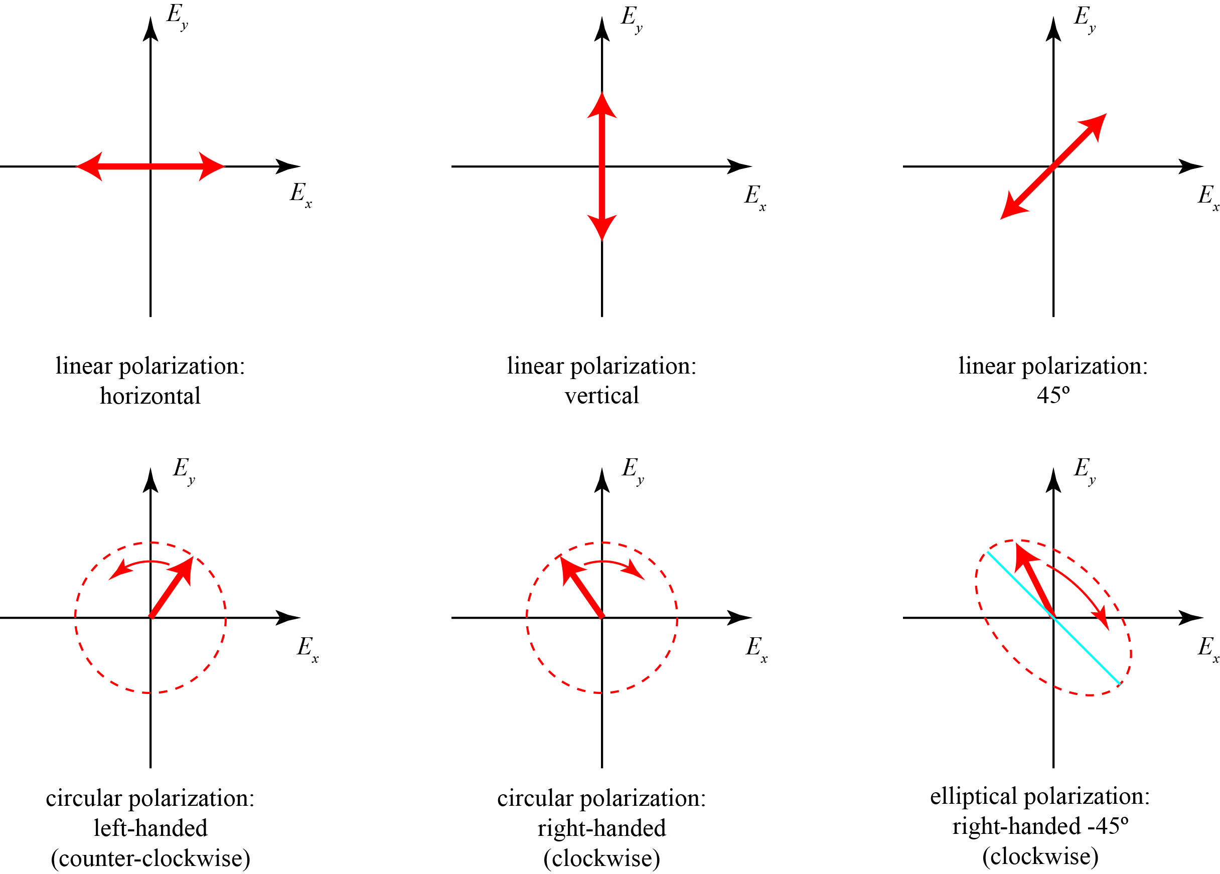
For linear polarization, the electric field vector just swings back and forth along a straight line. For circular polarization, the electric field vector goes in a circle, like the hands of a clock. For elliptical polarization, the electric field vector also circulates like a clock hand, but the length of the vector follows an elliptical path, rather than a circular path.

It’s worth nothing that the only important property of linearly polarized light is the angle that it is oriented. For circular polarization, the only important property is the handedness (which way it circulates). For elliptical polarization, however, there are three things to keep track of: the orientation of the ellipse, the handedness, and how elongated the ellipse is (called the ellipticity).

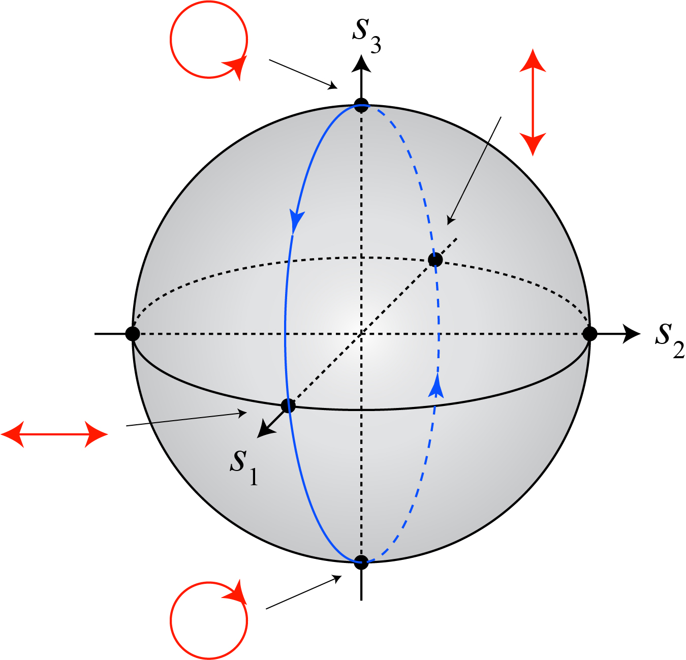
Basically, there are a lot of different ways the polarization can wiggle.  It’s a lot to keep track of, but in 1891 the brilliant mathematical physicist Henri Poincaré proved that every possible state of polarization can be associated in a meaningful way with a single point on a mathematical sphere, which is now called the Poincaré sphere.  A depiction of this mathematical sphere, with the different polarizations mapped out on it, is shown below.

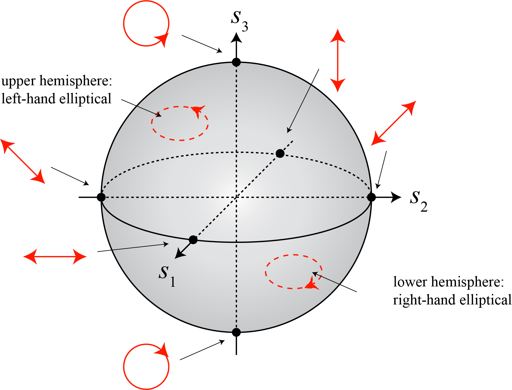
The North and South Poles of the sphere represent left-handed and right-handed circular polarization, respectively. The equator represents all possible states of linear polarization, with all orientations represented. Linear polarization has no handedness, and the equator ends up dividing the sphere into left-hand elliptical polarization (in the upper hemisphere) and right-hand elliptical polarization (in the lower hemisphere).

Before we continue, we should be a little more specific: the latitude on the sphere represents the amount of ellipticity, while the longitude represents the angle of the ellipse. If we draw a few representative cases up and down the sphere, we get the following picture.

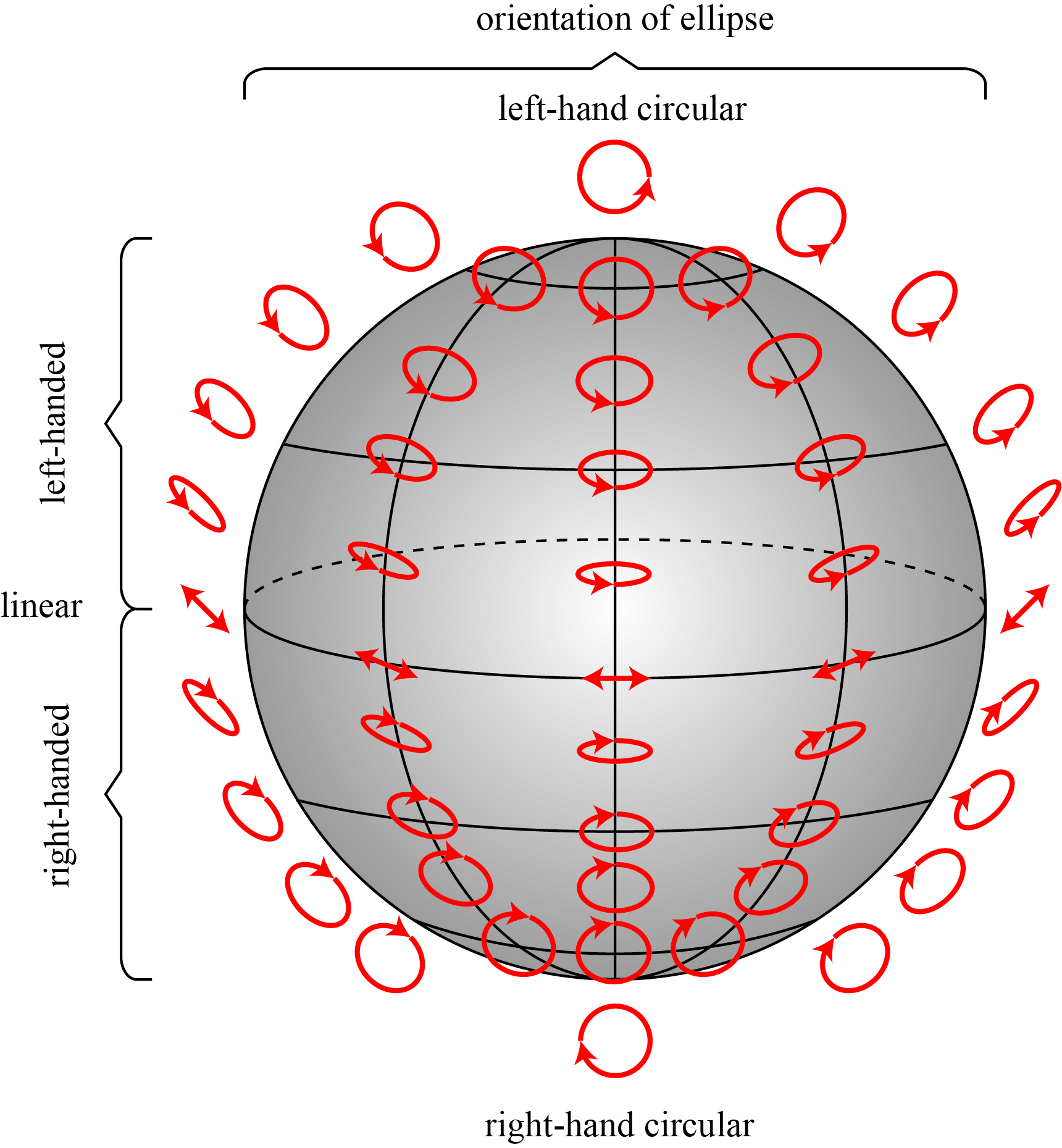
So if you were to go right down the front of the sphere, the left-handed circle would squash more and more until it became a horizontal line (linear polarization), and then as we went towards the South Pole, it would “unsquash” until it became a right-handed circle.

The Poincaré sphere is a very handy and elegant way to track the effects of different optical devices that a beam of light passes through. There are a variety of devices that can change the polarization of light; the most familiar of these is a polarizer, which blocks the wiggling of the electric field in one direction but allows the wiggling in a perpendicular direction.

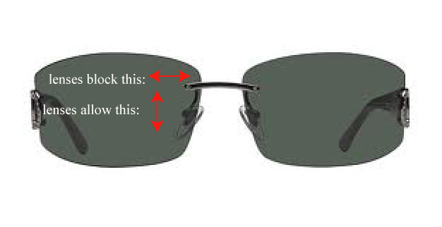
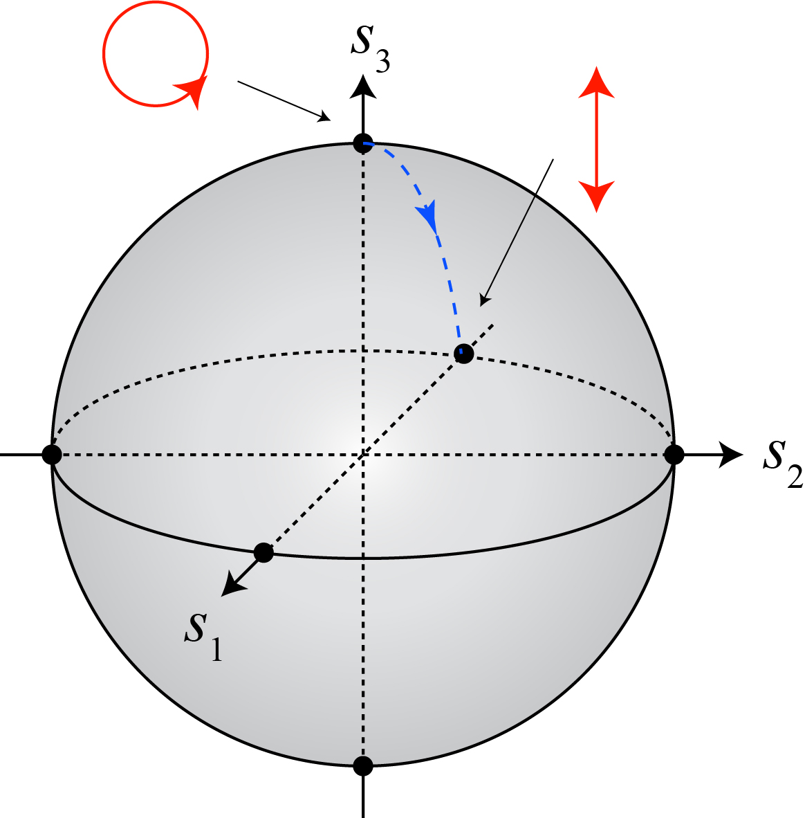
If we sent circularly polarized light through our sunglasses, then, our state of polarization would follow the path from the top of the sphere to back of the sphere, as all the horizontal wiggles are blocked and only the vertical wiggles remain.

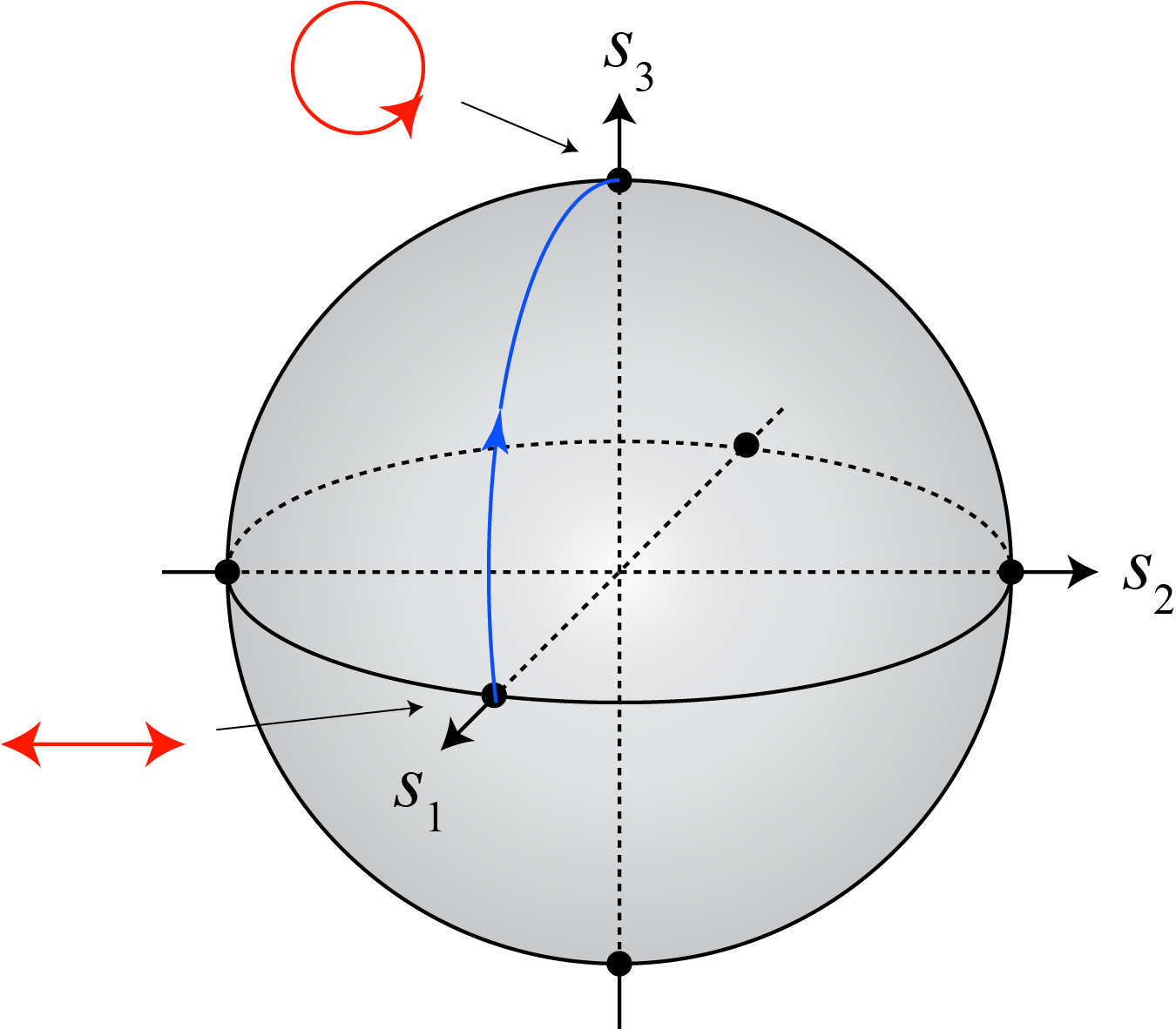
A second device we can use is called a rotator, which will rotate a state of linear polarization by a fixed amount. I’ve blogged about one way to create a rotator, which was discovered by Michael Faraday back in the 1800s!  If we imagine we start with vertical polarization, and use a rotator that rotates it to horizontal, then we get the path shown below.

A third device that is commonly used in optics is a quarter-wave plate.  If oriented properly, it can convert linearly polarized light into circularly polarized light, such as the path shown below.

You may have noticed that the three optical elements that I used made the state of polarization traverse a closed path on the sphere. The whole path is shown below.

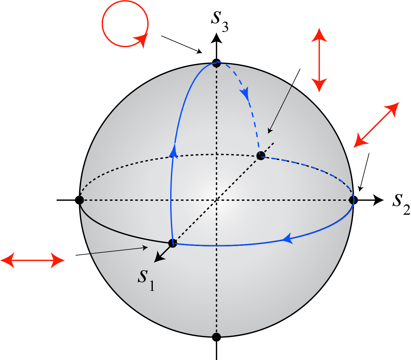
So, if we manipulate a light beam with the three optical elements mentioned previously, we take the beam of light from left-hand circular polarization, to vertical linear polarization, to horizontal linear polarization, and back to left-hand circular polarization. We’ve changed the state of polarization several times, but brought it back to its original state in the end.

But this is where it gets interesting! In 1956, Indian physicist Shivaramakrishnan Pancharatnam was studying how the state of polarization changes when light passes through crystals. He noticed that even when the polarization returned to its original state after manipulation, the light nevertheless was slightly changed. In particular, it had experienced an effective lag, or time delay, in its oscillation — what we call a change of phase.

The simplest picture of a wave that we can imagine is that it wiggles up and down as time passes, endlessly repeating. The “phase” of the wave refers to what point in its wiggle it is currently at.  Because the wave repeats itself, we define one full wiggle of the wave as 360 degrees, and the phase is some fraction of 360.

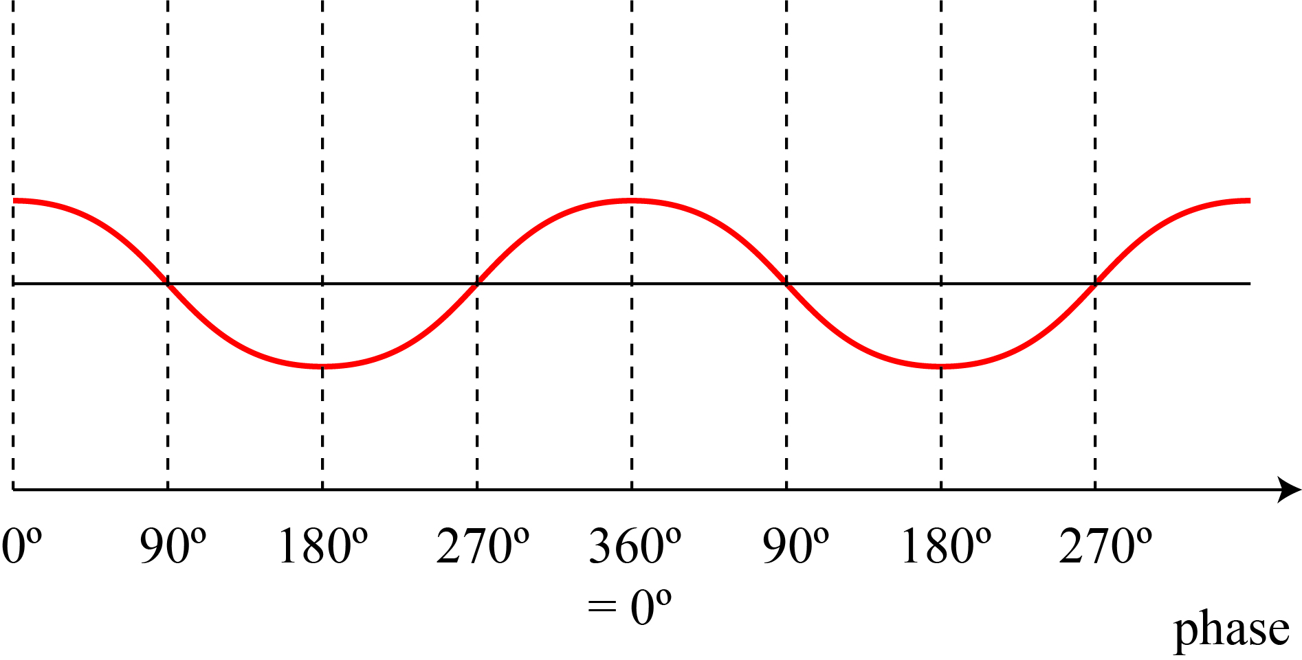
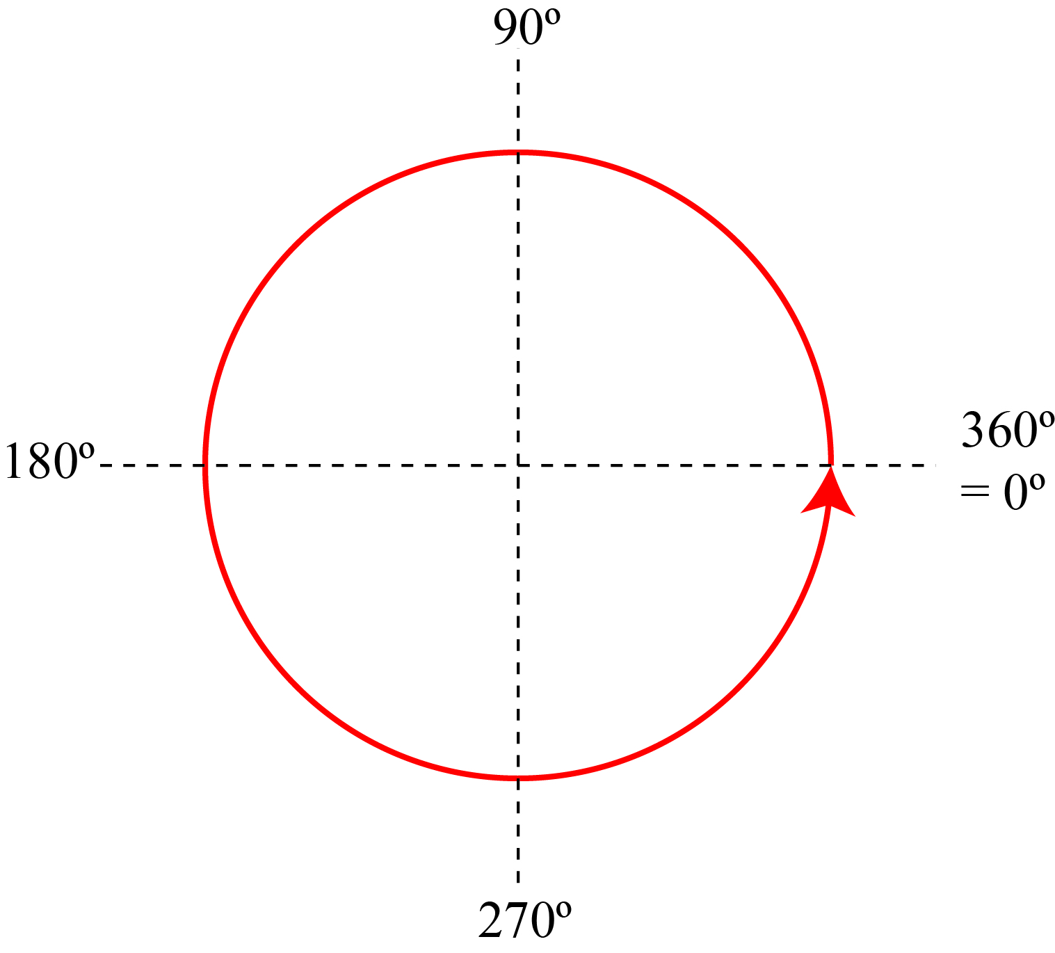
This picture is good for linear polarization, where the electric field vector swings back and forth, like a pendulum in a clock. For circular polarization, the electric field vector goes in a circle, like the hands of a clock. The phase in this case is just the position of the clock hand, which can also be measured in degrees.

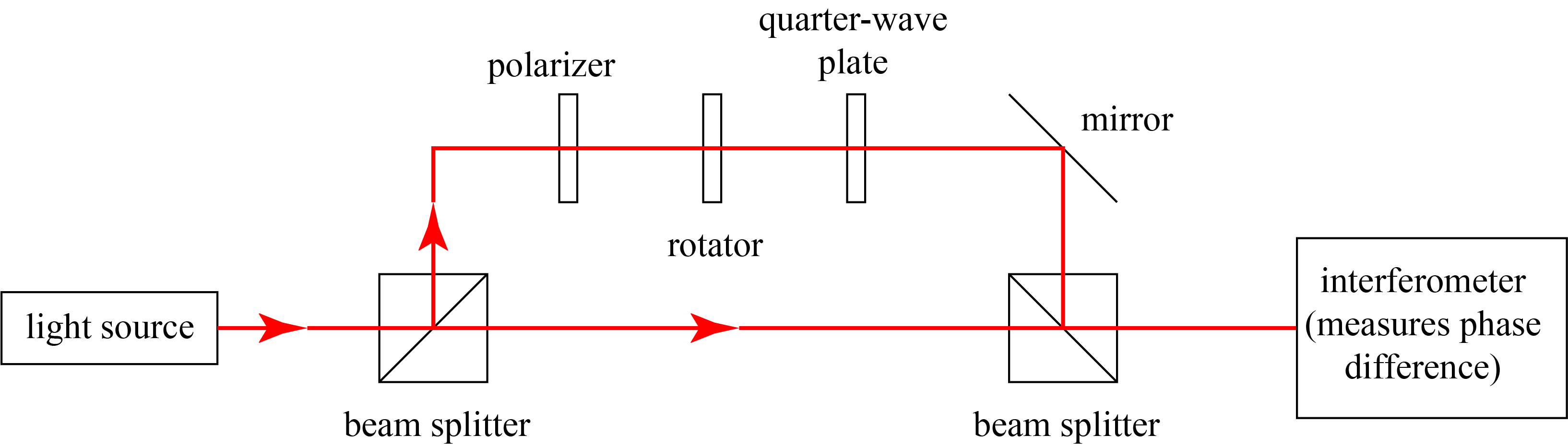
Pancharatnam compared the phase of a beam of circularly polarized light that had passed through a collection of optical elements, as shown above, to a beam of circularly polarized light that had remained unchanged and had passed through no elements.  An illustration of a hypothetical experiment is shown below. A single beam of polarized light is split into two. One beam goes through the optical elements, while the other does not. The two beams are combined, and their phase difference is measured using an interferometer (the details aren’t relevant to our discussion here).

Pancharatnam found, unexpectedly, that the phase of the manipulated beam of light was different from its unmanipulated counterpart. It is important to note that there are a number of factors that can change the phase relationship between the two beams: for example, if one beam travels a longer distance than the other, then the phase will be different. Also, light always slows down when traveling through an optical element, so its phase will be different from the phase of light that traveled the same distance through air. But, after accounting for these factors, Pancharatnam observed that there was an extra difference in the phase, a difference that was apparently due entirely to the manipulations of the state of polarization on the Poincaré sphere. He had found a phase purely due to the geometric manipulation of light: a geometric phase.

But where does this geometric phase come from?  Now we are at the climax of this post! Let us imagine the effect of our devices — polarizer, rotator, quarter-wave plate — on the actual polarization ellipse. We start with circular polarization, and put a black dot on the circle to indicate the current phase of the light (position on the circle).

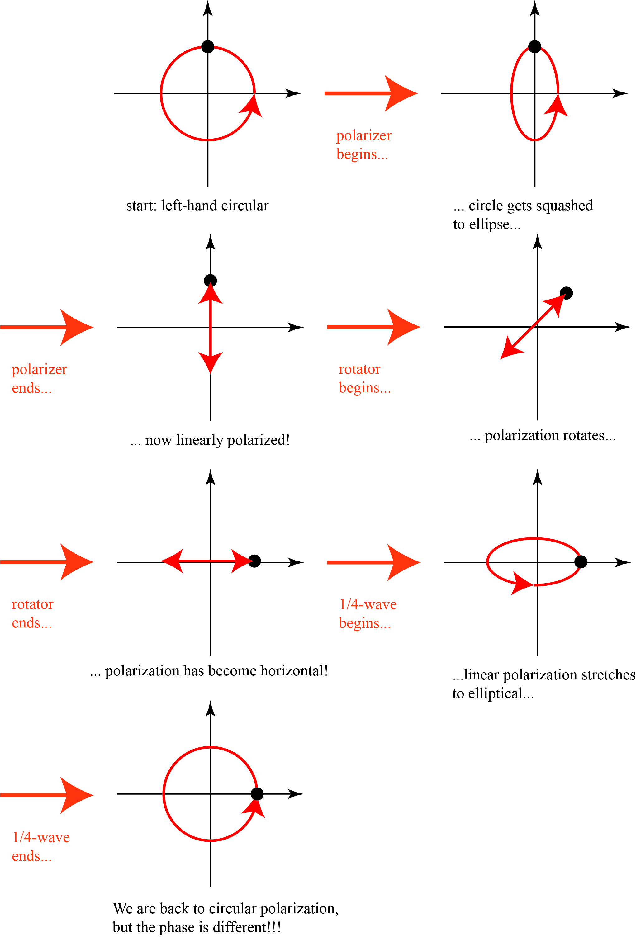
This picture illustrates the crux of the geometric phase: although we have returned to left-hand circular polarization at the end, we have effectively rotated the circle by our manipulations! This, to me, is the sense in which the phase is “geometric”: the change in the position of the phase (black dot) is entirely due to the geometric distortions of the polarization.

But there’s a real kicker to all of this: it turns out that the geometric phase can be calculated directly from the area enclosed by our path on the Poincaré sphere.  Rigorously, if we consider the total area of the sphere to be 720°, one can prove that the geometric phase is equal to 1/2 the area of our path on the sphere. For our example, the path enclosed is 1/4 of the total sphere, or 180°. One half of this is 90°, which is exactly the amount of phase change we found in our pictures above!

You may be doubtful of this relationship, so let’s look at one more example.  We now consider the following path on the Poincaré sphere.  We won’t bother describing how to do these transformations with optical elements: the beauty of the geometric phase phenomenon is that it only depends on the path, not what devices one uses to create the path!

In this case, our path cuts the sphere directly in half, so the area of one half of the surface (or the other) is 360°. The geometric phase must be half of this, or 180°.  Now let’s “calculate” the phase by manipulating the polarization ellipse, as before.

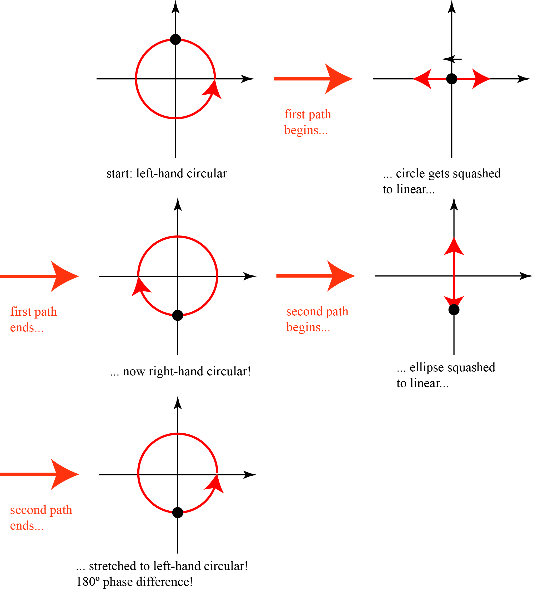
Our phase (black dot) ends up on the other side of the circle at the end, which is indeed 180 degrees!

Pancharatnam’s discovery was relatively unknown for many years. In the 1980s, however, Michael Berry discovered an analogous geometric phase in the behavior of quantum particles, and his colleagues in India pointed out Pancharatnam’s work to him. In optics, this phase is now referred to as the Pancharatnam phase.  As we’ve already noted, phases like this are found throughout physics — not only in optics and quantum mechanics, but in the swinging of a pendulum on the Earth and the flipping of a cat to land right-side up. In all cases, one finds that the initial and final positions of the system are the same, but that there is a “phase” of some sort that is different than it was initially. For Foucault’s pendulum, the difference is in the direction of the pendulum. For a falling cat, the difference is the cat is now right-side up instead of upside down.

The Pancharatnam phase has become a very important tool for designing novel, phase manipulating optical devices, such as flat lenses.  An ordinary lens, like those in eyeglasses or a telescope, manipulates the phase of light going through it by varying the thickness of the material. But it is now possible to cover a flat surface with a large number of tiny crystals, like those that Pancharatnam studied, where each crystal is oriented differently and consequently produces a differing Pancharatnam phase.  I don’t think it’s happened yet, but one day we all may have ultra-thin cameras where the lenses are designed using the ideas that Pancharatnam introduced some 60 years ago.