Note: This post is my contribution to The Giant’s Shoulders #2, to be held at The Lay Scientist. I thought I’d cover something a little more recent than my previous entries to the classic paper carnival; in truth, I need a break from translating 30-page papers written in antiquated German/French!

One of the fascinating things about scientific progress is what you might call its inevitability. Looking at the history of a crucial breakthrough, one often finds that a number of researchers were pushing towards the same discovery from different angles. For example, Isaac Newton and Gottfried Leibniz developed the theory of calculus independently and nearly simultaneously. Another example is the prehistory of quantum mechanics: numerous experimental researchers independently began to discover ‘anomalies’ in the behavior of systems on the microscopic level.

I would say that the development of certain techniques and theories become ‘inevitable’ when the discovery becomes necessary for further progress and a number of crucial discoveries pave the way to understanding (in fact, one might say that this is the whole point of The Giant’s Shoulders). Occasionally it turns out that others had made a similar discovery earlier, but had failed to grasp the broader significance of their result or were missing a crucial application or piece of evidence to make the result stand out.

A good example of this is the technique known as computed tomography, or by various other aliases (computed axial tomography, computer assisted tomography, or just CAT or CT). The pioneering work was developed independently by G.N. Hounsfield and A.M. Cormack in the 1960s, and they shared the well-deserved 1979 Nobel Prize in Medicine “for the development of computer assisted tomography.” Before Hounsfield and Cormack, however, a number of researchers had independently developed the same essential mathematical technique, for a variety of applications. In this post I’ll discuss the foundations of CT, the work of Hounsfield and Cormack, and note the various predecessors to the groundbreaking research.

What is computed tomography, and how does it work? CT is a technique for non-destructive imaging of the interior of an object. Its best-known application is in medical imaging, in which a portion of the patient’s body is imaged using x-rays, often to check for cancer. A picture of a modern CT scanner (from Wikipedia) is shown below:

The word tomography is derived from the Greek tomos (slice) and graphein (to write); it refers to the manner of image reconstruction: images of the body are put together in two-dimensional slices, which can then be assimilated into a full three-dimensional structure, if desired. An example of a CT image of the lungs is shown below (image from RadiologyInfo):

It is important to note that a CT image is far superior to a normal x-ray image such as one might get at the doctor’s office after breaking a bone (also from RadiologyInfo):

A standard x-ray, as shown above, is a single picture taken of a human ankle. The object to be imaged is placed between the x-ray source and a photographic plate, as schematically (and crudely) illustrated below:

Different materials in the human body absorb x-rays to a greater or lesser extent; bone absorbs the most. The image recorded on the photographic plate is in essence the x-ray shadow of the human body. This technique, though extremely useful for medical diagnosis, has a number of severe limitations. First and foremost, there is no depth information recorded about the object: the photographic plate records a ‘shadowgram’ of everything that lies between itself and the source. Small tumors could in principle be hidden (overshadowed) by a large piece of bone which lies directly above or below them. Second, a standard x-ray is extremely insensitive to soft tissue. As one can see in the ankle image above, the bone is clearly visible but the muscle and skin leaves hardly a trace on the plate. The technique will not detect a tumor in its earliest stages, which is the best time for successful treatment.

How does computed tomography differ? A computed tomogram is derived from a large number of x-ray shadowgrams, each taken at different angles of ‘attack’:

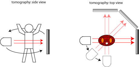
Each of these shadowgrams gives a different view of the interior of the patient’s body. By a nontrivial mathematical process requiring the use of a computer (hence the ‘computed’ in computed tomography), the information from this collection of shadowgrams can be combined to give a picture of a particular ‘slice’ of the body. Unlike a single shadowgram, this computed picture gives an exact cross-sectional picture of the body, and gives quantitative values for the absorption of different tissues of the body. Also unlike a single shadowgram, a CT scan can distinguish clearly between different types of soft tissue, as can be seen in the sample image above. A CT scan can find tumors at an earlier stage than a standard shadowgram.

We’ll discuss how CT actually works at the end of the post; for now, let’s look at the development of the process. The first work was done by Allan M. Cormack in the 1950s; in his own words (from his Nobel lecture),

In 1955 I was a lecturer in Physics at the University of Cape Town when the Hospital Physicist at the Groote Schuur Hospital resigned. South African law required that a properly qualified physicist supervise the use of any radioactive isotopes, and since I was the only nuclear physicist in Cape Town, I was asked to spend 1 1/2 days a week at the hospital attending to the use of isotopes, and I did so for the first half of 1956. I was placed in the Radiology Department under Dr. J. Muir Grieve, and in the course of my work I observed the planning of radiotherapy treatments. A girl would superpose isodose charts and come up with isodose contours which the physician would then examine and adjust, and the process would be repeated until a satisfactory dose-distribution was found. The isodose charts were for homogeneous materials, and it occurred to me that since the human body is quite inhomogeneous these results would be quite distorted by the inhomogeneities – a fact that physicians were, of course, well aware of. It occurred to me that in order to improve treatment planning one had to know the distribution of the attenuation coefficient of tissues in the body, and that this distribution had to be found by measurements made external to the body. It soon occurred to me that this information would be useful for diagnostic purposes and would constitute a tomogram or series of tomograms, though I did not learn the word “tomogram” for many years.

In simpler terms: radiation therapy requires being able to send a precise dosage of radiation to a particular location in a patient. The amount of radiation reaching a location in the body depends significantly on the internal structure, and no method existed at that time for measuring the absorption properties of an individual’s body; Cormack therefore decided to look for one. An initial literature search produced no prior results, so Cormack developed a mathematical technique for determining internal structure from a series of x-ray shadowgrams. The technique is now known as the Radon transform, and we will come back to it shortly.

Over the next few years, Cormack tested his new technique with systems, and targets, of increasing complexity. In 1957 in Cape Town he measured a circularly symmetric sample consisting of a cylinder of aluminum surrounded by an annulus of wood. As Cormack noted,

Even this simple result proved to have some predictive value for it will be seen that the three points nearest the origin [of his data set] lie on a line of a slightly different slope from the other points in the aluminum. Subsequent inquiry in the machine shop revealed that the aluminum cylinder contained an inner peg of slightly lower absorption coefficient than the rest of the cylinder.

By 1963, Cormack was prepared to do work on a “phantom” (simulated patient made of aluminum and lucite) without circular symmetry, using the device pictured below (taken from the Nobel lecture, again):

Quite a far-cry still from the CT machines of today, the cylinders are collimators containing the source, Co⁶⁰ gamma rays, and the detector. Quite good measurements of the properties of the phantom were found, and the results were published in a pair of papers in 1963 and 1964*. From Cormack’s Nobel lecture again,

Publication took place in 1963 and 1964. There was virtually no response. The most interesting request for a reprint came from a Swiss Centre for Avalanche Research. The method would work for deposits of snow on mountains if one could get either the detector or the source into the mountain under the snow!

Cormack did little else on this subject for a number of years. Meanwhile, about the time that Cormack was moving on to other things, Godfrey N. Hounsfield, working at EMI Central Research Laboratories in Hayes, UK, started thinking about the problem along similar lines. Now quoting from his Nobel lecture,

Some time ago I imagined the possibility that a computer might be able to reconstruct a picture from sets of very accurate X-ray measurements taken through the body at a multitude of different angles. Many hundreds of thousands of measurements would have to be taken, and reconstructing a picture from them seemed to be a mammoth task as it appeared at the time that it would require an equal number of many hundreds of thousands of simultaneous equations to be solved.

When I investigated the advantages over conventional X-ray techniques however, it became apparent that the conventional methods were not making full use of all the information the X-rays could give.

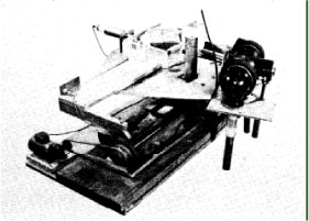
Hounsfield put together his own crude initial apparatus to test his ideas:

The equipment was very much improvised. A lathe bed provided the lateral scanning movement of the gamma-ray source, and sensitive detectors were placed on either side of the object to be viewed which was rotated 1” at the end of each sweep. The 28,000 measurements from the detector were digitized and automatically recorded on paper tape. After the scan had been completed this was fed into the computer and processed.

Many tests were made on this machine, and the pictures were encouraging despite the fact that the machine worked extremely slowly, taking 9 days to scan the object because of the low intensity gamma source. The pictures took 2 1/2 hours to be processed on a large computer… Clearly, nine days for a picture was too time-consuming, and the gamma source was replaced by a more powerful X-ray tube source, which reduced the scanning time to nine hours. From then on, much better pictures were obtained; these were usually blocks of perspex. A preserved specimen of a human brain was eventually provided by a local hospital museum and we produced the first picture of a brain to show grey and white matter.

Disappointingly, further analyses revealed that the formalin used to preserve the specimen had enhanced the readings, and had produced exaggerated results. Fresh bullock’s brains were therefore used to cross-check the experiments, and although the variations in tissue density were less pronounced, it was confirmed that a large amount of anatomic detail could be seen… Although the speed had been increased to one picture per day, we had a little trouble with the specimen decaying while the picture was being taken, so producing gas bubbles, which increased in size as the scanning proceeded.

The picture of Hounsfield’s prototype CT machine is shown below, taken from his Nobel lecture.

The use of fresh brains led to some entertaining moments, as he notes in his Nobel autobiography,

As might be expected, the programme involved many frustrations, occasional awareness of achievement when particular technical hurdles were overcome, and some amusing incidents, not least the experiences of travelling across London by public transport carrying bullock’s brains for use in evaluation of an experimental scanner rig in the Laboratories.

The initial tests demonstrated the principle, but a faster, more sophisticated machine needed to be built in order to make it a worthwhile clinical tool. By 1972 a machine similar in appearance to contemporary CT scanners was installed at Atkinson Morley’s Hospital, London, and was used on a woman with a suspected brain lesion. Hounsfield published a paper describing his new system, and naming it “Computerized transverse axial scanning tomography,” in 1973**.

The paper includes many technical details and a photograph of the various components, such as the basic machine, shown below:

This early machine had many differences with the machines of today. The early system took some five minutes to image a slice, but modern systems can finish such a scan in seconds. In the early system, a patient’s head was enclosed in a water-filled rubber cap, which reduced the range of x-ray intensities arriving at the detectors. The early system also, not surprisingly, had a relatively low resolution: pictures were 80 x 80 ‘picture points’, derived from 28,800 readings.

This work seems to have been immediately recognized as groundbreaking and of fundamental importance (at the very least this can be seen by how quickly the Nobel prize was awarded for the achievement). Most hospitals now have a radiology department with some sort of CT scanner. CT is also commonly used for nondestructive testing of materials in industrial applications. Applications involving other types of waves have also been applied: CT-like algorithms have been used in geological exploration and oil prospecting, as well as in magnetic resonance imaging (MRI), another important medical diagnostic technique. The same tomographic methods are now also used for reconstructing quantum wavefunctions (which is worth a post in itself at a later date). Techniques which are inspired by or generalize CT, such as diffraction tomography, diffusion tomography, and optical coherence tomography, are also in use or under investigation.

Perhaps more broadly, CT was the first widely successful application of the theory of inverse problems. An inverse problem is a solution of a physical problem in the opposite direction from the usual ’cause-effect’ sequence of events. Each inverse problem is associated with a more familiar ‘forward problem’ in physics which represents the ’cause-effect’ process. For instance, the problem of determining the absorption of x-rays given the structure which they are incident upon is a forward problem; the problem of determining the structure of an object based on how x-rays are absorbed by the object in an inverse problem. Computed tomography effectively created its own ‘inverse problems’ subfield of mathematical physics.

Interestingly, though, the mathematical problem solved by Cormack turns out to have been solved numerous times previously by other researchers for other applications though, as noted at the beginning of this post, those works either were too far ahead of their time or too limited in application to gain much attention. All of these were acknowledged by Cormack in his Nobel lecture.

The first to develop the mathematics behind computed tomography was Johann Radon*** in 1917, in his paper, “Über die Bestimmung von Funktionen durch ihre Integralwerte längs gewisser Mannigfaltigkeiten.” (“On the determination of functions by their integral values along certain manifolds”.)

In probability theory, the problem was developed by H. Cramér and H. Wold in 1936****. In 1968, D.J. De Rosier and A. Klug***** used a similar technique in electron microscopy to reconstruct the three-dimensional structure of the tail of a bacteriophage, work which eventually led Klug to win the 1982 Nobel Prize in Chemistry “for his development of crystallographic electron microscopy and his structural elucidation of biologically important nucleic acid-protein complexes.”

Perhaps the most unusual precursor to computed tomography is the 1956 work by R.N. Bracewell******, who derived exactly the same mathematical technique to reconstructions of celestial radio sources.

Enough history, for now: how does computed tomography (and its predecessors) work? The exact mathematics of CT, i.e. Radon’s elegant formula for reconstruction an object, is rather involved, and will be left for a future post. Instead we give two simple illustrations of the principles behind the process, one completely conceptual and one which involves a little bit of math.

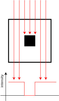
First, a conceptual illustration: suppose we have a ‘black box’ which contains a perfectly absorbing object inside of it. We wish to roughly determine the shape of that object by measuring the absorption of x-rays which pass through the box. Let’s pretend that the object within the box is a square; how many measurements do we need to prove this? Suppose we first shine x-rays horizontally through the box; the result is as follows:

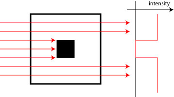
The intensity of the x-rays as a function of position is plotted on the right. This clearly doesn’t tell us the shape of the object, because the following objects would result in the same shadow:

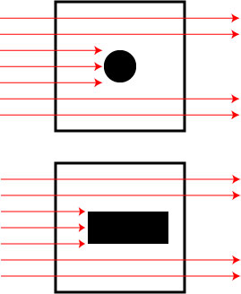
We can eliminate the possibility of the rectangular shape by shining our x-rays from above:

This second measurement still, however, cannot distinguish between a square object or a round object. We can then take a diagonal measurement:

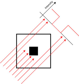
This measurement suggests that the object is wider along the diagonal, but we are still left with the following possibility for an object:

By making even more measurements, we can narrow down the shape of the object. In a realistic CT measurement, there are no ‘perfectly absorbing’ objects, but the same principle applies: by measuring the absorption properties of the patient/target from many directions, one can develop the interior absorption profile of the object.

Obviously, determining the actual absorption profile from the massive amount of x-ray data is not a trivial process. Radon (and Cormack’s) theoretical formulation of the problem describes how the x-ray data is related to the object absorption. With the help of a computer, one can substitute the data into Radon’s formula to get an exact description of the object’s properties.

Let’s try and show how tomography works in another, more algebraic, way: suppose we reduce our ‘patient’ to a block of 9 different regions, each with its own absorption coefficient :

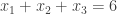
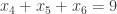
We wish to determine each of these numbers, but the only way we can measure them is by passing an x-ray through the box and measuring the total of any row, column, or diagonal; for example:

According to basic linear algebra, in order to uniquely solve a system of equations for 9 unknowns ( the ), we need 9 independent equations relating those unknowns. We make the following ‘measurements’ through the box, with the following results:

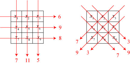
This gives the following set of 12 equations:

, , ,

, , ,

, , ,

, , .

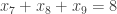
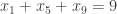
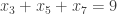
It turns out that we need 11 of these equations to solve uniquely for the values within the squares, as the equations are not independent of one another. This can be seen by noting that the sum of the first three equations gives

,

which is exactly the same equation as the sum of the second three equations,

.

Using a computer to solve the equations, the numbers within the boxes are:

If we have a larger system of boxes, we will need even more measurements to make a unique solution. In the idealized limit of an infinite (continuous) set of boxes, we would need to measure the transmission through the square from every direction.

This ‘brute force’ method of doing tomography was in essence the solution used by Hounsfield in his original paper, as he was unaware of the work of Radon and Cormack; he notes:

If the body is divided into a series of small cubes each having a calculable value of absorption, then the sum of the absorption values of the cubes which are contained within the X-ray beam will equal the total absorption of the beam path. Each beam path, therefore, forms one of a series of 28,800 simultaneous equations, in which there are 6,400 variables and, providing that there are more equations than variables, then the values of each cube in the slice can be solved. In short there must be more X-ray readings than picture points.

We can see that this method is inefficient even from our simple example, as we ended up having more measurements than we needed. The use of Radon’s née Cormack’s formula gives a better understanding of how to sort, arrange, and efficiently process the acquired data.

The history of Cormack and Hounsfield’s discovery makes a good argument by example for the usefulness of ‘cross-pollination’ between fields and subfields of science. Radon’s original calculation had to be ‘rediscovered’ numerous times by different authors working in different fields, a process which is not uncommon in the physical sciences.

On the flip side, authors often make major breakthroughs or simplify their work greatly by searching for results which have been forgotten or restricted to a little-explored subfield. The now hot topic of metamaterials began in essence with the rediscovery of a 1967 paper by Russian scientist V. Veselago. The field of quantum optics was advanced rapidly by applying results that had already been developed in the field of nuclear magnetic resonance.

None of this should be taken as a slight on the achievements of Cormack and Hounsfield; they saw possibilities in the development of tomographic methods that numerous others who came before them did not. Their researches came at a time when there was a genuine need for new diagnostic techniques, coupled with the computational ability to carry them out.

**************************************

* A.M. Cormack, “Representation of a function by its line integrals, with some radiological applications,” J. Appl. Phys. 34 (1963), 2722-2727. A.M. Cormack, “Representation of a function by its line integrals, with some radiological applications. II,” J. Appl. Phys. 35 (1964), 2908-2913.

** G.N. Hounsfield, “Computerized transverse axial scanning (tomography): Part I. Description of system,” Brit. J. Radiol. 46 (1973), 1016-1022.

*** J. Radon, “Über die Bestimmung von Funktionen durch ihre Integralwerte längs gewisser Mannigfaltigkeiten,” Ber. König Säch. Aka. Wiss. (Leipzig), Math. Phys. Klasse 69 (1917), 262-267.

**** H. Cramér and H. Wold, “Some theorems on distribution functions,” J. London Math. Soc. 11 (1936), 290-294.

***** D.J. De Rosier and A. Klug, “Reconstruction of three dimensional structures from electron micrographs,” Nature 217 (1968), 130-134.

****** R.N. Bracewell, “Strip integration in radio astronomy,” Austr. J. Phys. 9 (1956), 198-217.