This is part 2 in a lengthy series of posts attempting to explain the idea of quantum entanglement to a non-physics audience.  Part 1 can be read here.

So, by the mid 1920s, physicists had made significant progress in developing the new quantum theory.  It had been shown that light and matter each possess a dual nature as waves and particles, and Schrödinger had derived a mathematical equation that accurately described how the wave part of matter evolves in space and time.

But it was not clear what, exactly, was doing the “waving” in a matter wave.   Water waves arise from the oscillation (waving) of water, sound waves arise from the oscillation of molecules in the air, but what is oscillating in a matter wave?  Or, to put it another way, what does such a wave represent?

We will try and answer this question by looking at how a matter wave manifests in an actual experiment.  It turns out that the best example for demonstrating the wave properties of matter is also the best example for demonstrating the wave properties of light: Young’s classic double slit experiment!  However, the double slit experiment was not done with electrons until decades after the foundation of quantum mechanics, so we must briefly step away from our historical discussion to investigate it.

For light, the double slit experiment was conceived by Thomas Young in 1804, and it was the first definitive proof that light behaves as a wave.  His experimental setup is roughly illustrated below.

Light from a source is used to illuminate a pair of closely-spaced slits in an opaque screen S.  The light that emerges from the pair of slits spreads out in all directions, like ripples spreading from a rock thrown in a pond.  The waves from the two slits interfere with one another, forming regions of light and darkness; these regions are projected on a measurement screen M.  Thomas Young’s beautiful illustration of this effect is shown below.

Young’s original image of the double slit experiment, showing waves emitting from the two slits combining Points C,D, E and F would be dark  on the measurement screen.

Where the ripples from the two slits overlap, the waves add together, producing a bright region.  Where the ripples do not intersect, the waves cancel out, producing a dark region.  Points C, D, E and F in Young’s figure represent dark regions.

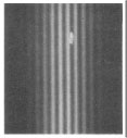
If this is not clear, the result of the experiment is that the light tends to form bright bands on the measurement screen, separated by regions of darkness; a crude simulation of how this would appear on the screen is shown below, assuming that the slits are horizontally side-by-side.

As we have said, Young’s experiment can also be done with electrons!  The wavelength of the electrons is much, much smaller than the wavelength of light, which means that the slits must be much closer together to get an observable interference pattern, but fundamentally the experiment is the same.  It was first performed in 1961 by Claus Jönsson¹, and his image of the detected electrons is shown below.

Electron interference pattern from 1961 experiment.

So far, there is nothing noticeably different from Young’s experiment with light — we have the same interference pattern, but the bright lines are caused by electrons instead of photons.

But Jönsson’s experiment used a constant stream of electrons; what happens if electrons are sent one at a time towards the two slits?  It is important to note that Schrödinger’s equation, which describes the wave properties of matter, applies to a single electron; we should therefore somehow see wave effects in such a case, but how do they manifest?

Such a modified experiment has been done a number of times, but one of the most elegant versions was done by A. Tonomura, J. Endo, T. Matsuda, T. Kawasaki and H. Ezawa² in 1989.  They sent the electrons through the system one by one, and tallied the locations where they hit the screen.  Images of the measurement screen are shown below.

Left to right, top to bottom, shows the accumulation of electrons as time passes.  We make a number of observations from these images:

• Individual electrons appear as points on the screen, not as waves.  Evidently the electrons appear as localized particles when we measure their position.
• Individual electrons arrive somewhat randomly on the screen.  It is not possible to predict exactly where any particular electron will arrive.
• When we look at the arrival of many, many electrons on the screen, we find that they reproduce the familiar wave interference pattern of Young’s experiment!

This is a bewildering set of observations.  Let us focus on the second and third points first.  Apparently, it is not possible to say with certainty where any particular electron will arrive, but electrons are more likely to arrive at places where the wave is strong, and unlikely to arrive at places where the wave is weak.  Apparently, the matter wave of a quantum-mechanical particle such as an electron should be interpreted as relating to the probability of finding the particle at that point in space.

So, the answer to “what does a matter wave represent?” is, apparently: “a wave of possibilities.”

This idea, that the amplitude of a matter wave is directly related to the probability of finding the particle in that location, was originally stated by German physicist Max Born in 1926, and is now known as the “Born rule“.  This was a profoundly new way of thinking about nature, and it led to Born winning 1/2 of the 1954 Nobel Prize in Physics.

Before we continue, we should note that there is a similar relationship between a light wave and the behavior of the photons in that wave.  This was demonstrated elegantly in 2007 by T.L. Dimitrova and A. Weis³; they performed Young’s double slit experiment with a severely attenuated light beam, such that photons passed through the system one at a time.  Their integrated result appears below, and is more or less indistinguishable from the electron case!

This behavior, exhibited by both matter and light, suggests that there is an inherent randomness to the behavior of elementary particles, and this idea was radical when Born suggested it. Before Born’s time, physics was assumed to be a deterministic science. That is: it was assumed that we live in a “clockwork universe,” whose pieces were set into motion at the beginning of time and have been moving predictably in accordance with the laws of physics ever since.

Born’s argument changed that.  It suggests that the laws of physics themselves have randomness built into them.  Even if we send two electrons through the same double slit experiment in exactly the same way, we cannot say with certainty where each of them will end up on the measurement screen.  The best we can do is say where any individual electron is likely or not likely to appear.

Such a huge change to the philosophy of physics raised additional questions, and problems.  Among them:

• Where is the electron during the time it is emitted from the source until it arrives as the measurement screen?
• What makes the electron “choose” where to hit the measurement screen?

These questions were pondered by Niels Bohr and his assistant Werner Heisenberg at Bohr’s institute in Copenhagen over the years 1925-1927.  The outcome of their pondering became known as the Copenhagen interpretation of quantum mechanics and, in the context of Young’s experiment, we can describe it as follows:

• When the electron is emitted and traveling through the double slit experiment, it evolves as a wave in accordance with Schrödinger’s equation.
• While traveling as a wave, the electron has no definite position: it is, in a sense, taking every possible path through the system simultaneously.  The electron goes through both slits!
• When the electron arrives at the measurement screen, i.e. it is measured, it “chooses” where to appear, with probabilities as given by the Born rule.  The wave “collapses” and the electron is observed in a definite location.

This interpretation of quantum physics is consistent with experimental observations.  Philosophically, however, it is rather a bit of a mess.  The biggest problem lies with this idea of “measurement” and the “collapse of the wavefunction.”  Bohr and Heisenberg roughly defined a “measurement” as an interaction of the quantum particle with a researcher’s detection apparatus.  This is vague, however, and seems to imply that human beings play a unique role in quantum physics: that quantum particles exist in this uncertain wave state until we, as humans, observe them.  Physicists had spent centuries demonstrating that human beings are bound by the same laws of physics as every other object in the universe, so this was an unwelcome step backwards.

The collapse of the wave upon measurement poses its own problem. Schrödinger’s equation, which describes how a matter wave evolves, does not include any mechanism for this collapse.  Wavefunction collapse is, in essence, rather crudely duct-taped onto the quantum theory, with no rigorous theoretical model for it.

The problems with measurement and wavefunction collapse have led to a mantra and joke among physicists working in quantum theory: “shut up and calculate.” In other words: don’t ask whether the theory actually makes sense, just use it to predict and understand experimental results.

So, by the late 1920s, the model of quantum physics could be summarized as follows.  Quantum particles travel throughout space as a probability wave, with no definite position, until they are measured by an experimental apparatus.  When measured, the particle “chooses” a definite position based on the probability wave amplitudes and the wave “collapses” into that definite position.

This view of how quantum physics works, however, leads to very strange predictions when two or more quantum particles have a relationship with each other.  This is what we will know as quantum entanglement, which we will at last introduce in Part 3 of this series of posts!

POSTSCRIPT: The Copenhagen interpretation is not the only way to interpret experimental results in quantum physics.  Other models include the “many worlds” interpretation, and the “pilot wave” interpretation.  For our purposes, however, Copenhagen is the easiest way to think about things for the moment.

***************************************

¹  C. Jönsson, Zeitschrift für Physik 161 (1961), 454. Reprinted in English as “Electron diffraction at multiple slits,” Am. J. Phys. 42 (1974), 4- 11.

² A. Tonomura, J. Endo, T. Matsuda, T. Kawasaki and H. Ezawa, “Demonstration of single-electron buildup of an interference pattern,” Am. J. Phys. 57 (1989), 117-120.

³ T.L. Dimitrova and A. Weis, “The wave-particle duality of light: A demonstration experiment,” Am. J. Phys. 76 (2008), 137-141.