
This is part 3 in a lengthy series of posts attempting to explain the idea of quantum entanglement to a non-physics audience. Part 1 can be read here, and Part 2 can be read here.
Here, in part 3, we will at long last introduce entanglement! But, before we do, we need to be sure we really understand what the wave properties of a quantum particle imply about its behavior.
So, by the late 1920s, physicists knew that discrete bits of matter — electrons, for example — sometimes act like a wave and sometimes act like a particle. This seemingly contradictory nature is often referred to as wave-particle duality. It was not immediately obvious how to interpret the wave properties of matter, but physicists finally settled on what is referred to as the “Copenhagen interpretation,” after the city in which it was more or less developed. If we consider the motion of a single electron, the Copenhagen description of quantum behavior could be summarized as follows:
- While freely propagating through space, the electron and all of its properties evolve as a wave.
- The wave may be described as a “wave of possibilities”: the amplitude of the wave only describes the probability of the electron to be found in a certain position or configuration.
- While evolving as a wave, the electron in general has no definite position or configuration — it is, roughly speaking, existing in all possible configurations simultaneously. In Young’s double slit experiment, for instance, it is often said that the electron goes through both slits.
- When a property of the electron is measured in an experiment, where the property must take on a definite value, the electron “chooses” an outcome, based on the wave probabilities mentioned above. The wave “collapses” into that single outcome. For instance, if we have a detector to measure the position of the electron, we will see that electron at a single definite location on the detector.
- If the particle still is free to continue moving, the process repeats itself, the collapsed wave evolving again, usually resulting in a wave of many possible outcomes again.
You might have noticed that I have sneakily added the word “configuration” when describing the behavior of the electron. In previous posts, we have described the electron as being a wave that evolves in space and time, implying that the wave describes the probability of finding the particle in a particular place at a particular time. However, every aspect of a quantum object is similarly wrapped up in this “wave of possibilities,” and is uncertain until it is specifically measured. This includes the energy of the particle, the momentum of the particle and, what will be particularly important to us, the angular momentum of the particle. We usually refer to the entire collection of properties of the particle that can be known simultaneously as the state of the particle.
At this point, all of this talk of “measurement” and “probability” might seem a little abstract. Let us try and make it clear with a silly example: a quantum quarter!

Yes, one of these.
Let us imagine that we are able to fabricate a really, really small quarter, of a size comparable to that of an atom. Then this quarter would be subject to the laws of quantum physics, and the Copenhagen interpretation applies. Let us imagine we flip this quantum coin — what happens?
- After the flip, but before looking at it, the quantum quarter is in a wave state that is simultaneously 50% heads and 50% tails.
- When we look at the coin, i.e. when we measure it, the quarter “chooses” one of the outcomes, and becomes either definitely heads or definitely tails.
The key difference between this quantum coin flip and an ordinary coin flip is in the first part of this description. When we flip an ordinary coin, we may not know the outcome — we covered the coin with our hand, for instance — but it is definitely either heads or tails under our hand. With the quantum quarter, it is heads and tails until we look at it and “collapse” the wave of the quarter.
At this point, it will be helpful to introduce a little mathematical notation. We aren’t going to do any complicated mathematics here, but the notation will make the discussion a little clearer. First of all, let me represent the state of the quarter, after being flipped but before being looked at, as follows.

This looks a little strange at first, but I have written the state of the quarter in exactly the form that a quantum physicist would. The combination |〉 symbolizes the quantum state of an object; by |quarter〉 we mean “the general quantum state of the quarter.” aheads represents the amplitude of that part of the wave which represents the quarter landing on heads, and atails represents the amplitude of that part of the wave which represents the quarter landing on tails. The objects |heads〉 and |tails〉 represent the quarter being either heads up or tails up.
Our equation written above, then, states that “the quantum state of the quarter (before measurement) is a combination of the quarter being in the state heads up and the state tails up.”
If it is a fair quarter, we expect that the probabilities of heads or tails are equal, i.e. 1/2 for each. (Where we use 1 = 100% and 1/2 = 50%.) Our quantum state of the quarter may then be written as:
Whenever we describe the state of a particle as being some sum of distinct outcomes, we refer to it as a superposition.
Wait: why is it one over the square root of two, instead of 1/2? You may remember in a previous post that I mentioned the Born rule for relating the quantum wave of the system to the probability of a particular measurement; it turns out that the relation between the probability p of a particular outcome and the amplitude a of that outcome in the wave is:

We don’t need to worry about this too much in our discussion going forward, but I wanted to write the equation in its physically correct form.
So what happens to the quantum state of the quarter after measurement? We cannot predict with certainty what happens: the Copenhagen interpretation of quantum mechanics implies that the outcome is truly a random one. Let us suppose we find that the quarter is heads up; this means that the quantum state of the quarter has “collapsed” to the form

The part of the state that was |tails〉 has disappeared, leaving us with a quantum quarter that is definitely, 100% heads up.
If this idea of “wavefunction collapse” seems strange and somewhat unsatisfying to you, you’re not alone: this part of quantum physics troubles and confounds researchers to this day. Nowadays, the conundrum is known as the “measurement problem.” We will talk a lot about this in the near future, but let me just point out one issue with the idea of “measurement” right now: what counts as a measurement? The way we have described it, it sounds as if a human being observing a quantum particle is necessary for the wave to collapse. This is, however, clearly an unsatisfactory explanation, as there is no reason to think that humans, or any living creatures, have such a special influence on the state of reality. Such an interpretation of wavefunction collapse is more an indication of our human-centric bias in describing the universe than any profound physics.
A slightly better explanation is that a measurement occurs whenever a quantum particle like an electron interacts with a macroscopic system, i.e. any laboratory detectors. The thinking here is that, somehow, a large collection of atoms or other quantum particles act fundamentally different than a small number, and that the large collection forces the electron to “make up its mind,” so to speak. Call it a quantum-mechanical form of peer pressure, if you will! This is also not particularly satisfying, and we will have more to say about measurement going forward.
Now we are finally, finally ready to introduce entanglement! Let us do so by sticking with our quantum quarter example; however, we now consider the situation where we glue two quarters together, tail to tail. This means that the heads of the two coins are facing outwards. In what is a subtly important point, we scratch a number “1” on one of the outward faces of our double coin, and a number “2” on the other, so that the two faces are distinguishable. This is more or less what the system looks like:
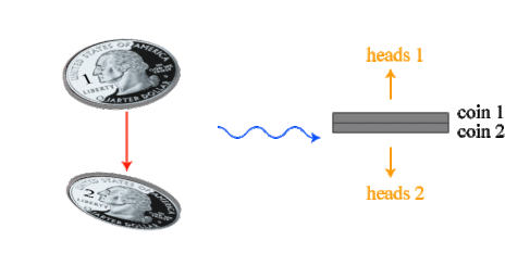
Let’s think about the outcomes of a non-quantum version of this first. If we flip the coin and it lands with heads 1 up, that means that tails 2 is up; similarly, if heads 2 lands facing up, that means that tails 1 is up. These are the only two possibilities from the flip of this double coin: the two coins, by nature of their gluing, always land with opposite faces up.
Similar to our earlier argument, the flip of this non-quantum double coin lands with “heads 1, tails 2” or “tails 1, heads 2”. If we were to make a quantum version of this coin, then, before it is measured, it is in the state “heads 1, tails 2” and “tails 1, heads 2”. In terms of our quantum physics notation, we may write:

This is our first example of quantum entanglement. It should be noted that it is not possible to talk about the quantum state of quarter 1 without taking into account the behavior of quarter 2, because the behaviors of the two coins have a definite relationship to each other: their fates are “entangled,” somewhat like the fates of two prisoners chained together at the wrist are entangled!

The 1958 movie The Defiant Ones, in which two shackled prisoners must work together to survive.
A rough way of thinking about entanglement is that it arises when the physics of a problem forces a definite relationship between two quantum objects but does not force either object to take on a definite state. For our quantum double quarter, the two coins will always land with opposing faces pointing upward, but nothing predetermines whether it will be coin 1 or coin 2 that lands heads up.
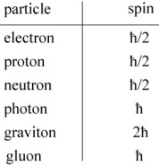
Our idea of a “quantum coin” and “quantum double coin” may seem quite artificial, but it turns out that electrons and other elementary particles such as protons and neutrons possess a property somewhat analogous to it, known as spin†.
You are hopefully familiar with the concept of angular momentum, which may be roughly described as the “momentum of rotation.” Such angular momentum is usual broken into two types: orbital and spin. As the name implies, orbital angular momentum comes from the orbital motion of an object around some external axis of rotation, while spin angular momentum comes from the rotation of an object about its own axis. The motion of the Earth around the Sun has orbital and spin components, as roughly illustrated below.

The spin axis of the Earth is in fact tilted, but I didn’t bother to add that detail to this image.
The spin of quantum particles is a little different: the measured spin of an elementary particle is a fixed quantity that never changes, and is either an integer or half-integer multiple of Planck’s constant, “h-bar.” The spin of some elementary particles is tabulated below; we will often write “spin-1/2” as shorthand for 
Even stranger: the spin of a spin-1/2 particle like an electron will always be measured as either +1/2 or -1/2. That is, the spin of the particle is 1/2 but it can be measured as spinning in a clockwise sense or a counterclockwise sense, which we refer to as “spin-up” or “spin-down.”
You may see where we’re going with this now: a spin-1/2 particle acts very much like a quantum quarter! The mathematical formula for such a state can be written as:
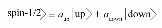
This can be read as “the general quantum state of a spin-1/2 particle is a superposition of a spin-up state and a spin-down state.”
We may also create an entangled spin state between two quantum particles by using the conservation of angular momentum. Let us suppose that we have an unstable, zero electric charge, spin-0 particle such as a pion which decays into a negatively-charged electron and a postively-charged anti-electron (positron), as crudely illustrated below.

Because the total angular momentum of the system is conserved, the net spin momentum of the electron and positron together must equal zero, which was the spin of the pion. This means that if the electron is spin-up, the positron is spin-down, and vice-versa. However, there is nothing in the laws of physics that forces either the electron or the positron to be spin-up or spin-down, so the quantum state of the electron and positron together must be a superposition of both possibilities: we have an entangled state almost exactly like the double quarter from earlier!

We may interpret this equation¹ as saying that “the two spin-1/2 particles end up in a quantum state which is an equal superposition of the positron being spin-up and the electron being spin-down with the positron being spin-down and the electron being spin-up.”
As in the double quarter case, we expect that if we measure the electron as being in a spin-down state, then the wavefunction has collapsed so that the positron is definitely in the spin-up state. There is one huge difference between the electron-positron case and the double quarter case, however. The quarters were stuck together, and physically connected to each other; the electron and positron, however, can be allowed to propagate through space an arbitrary distance away from each other without measuring them. Then, in principle, the quantum state written above still holds even when the electron and positron are light-years away from each other; what happens when we measure the spin of, say, the electron?
Let us suppose that it is measured to be spin-up. According to the Copenhagen interpretation, the entire wavefunction immediately collapses into the spin-up state of the electron. However, because of angular momentum conservation, the positron must have instantly collapsed into the spin-down state. This collapse must, evidently, happen instantaneously, that is, faster than the vacuum speed of light; otherwise, a measurement of the positron in the meantime could also return a spin-up value, which would violate angular momentum conservation!² At first glance, then, it would seem like quantum entanglement allows violation of the universal speed limit that Einstein’s theory of relativity postulates.
This idea, which implies that entanglement allows the quantum state of separated particles to change instantaneously when one of them is measured, was referred to by Albert Einstein as “spooky action at a distance.” This phrase was not intended to be flattering. In a paper published in 1935, Einstein, Podolsky and Rosen³ (EPR) used “spooky action” to argue that the Copenhagen interpretation of quantum mechanics, and the idea of “wavefunction collapse,” must be incorrect.
In the Copenhagen interpretation, as we have seen, the behavior of a quantum particle or particles is truly random: that is, it exists in a superposition state, both spin-up and spin-down simultaneously, until it is measured, at which point it chooses an outcome. EPR instead concluded that the seeming randomness of a quantum system is simply a symptom of the fact that we do not know how to properly measure all the factors that determine whether a particular particle is spin-up or spin-down. The situation, they argued, is very much like the flipping of an ordinary coin. We treat the flipping of a coin as a random event, but in fact if we were able to properly measure all the variables of the flip — how high we tossed the coin, how much we made it spin, how much it will bounce on landing — we would be able to know with 100% certainty whether it will come up heads or tails. It only seems random because we don’t usually measure, or know how to measure, all the variables that decide whether a coin comes up heads or tails.
Similarly, EPR said that quantum particles like electrons must possess “hidden variables” that determine whether the particle is measured spin-up or spin-down. The process seems random to us, but that is only because we don’t know what those additional variables are. EPR argued that the state of the electron and positron are always perfectly well-defined, in contrast to “wave of possibilities” that the Copenhagen interpretation suggests.
Another objection to the Copenhagen interpretation of quantum physics was suggested in 1935 by Schrödinger4, and it is also intimately connected to the measurement problem we discussed earlier. As he tells it:
One can even set up quite ridiculous cases. A cat is penned up in a steel chamber, along with the following diabolical device (which must be secured against direct interference by the cat): in a Geiger counter there is a tiny bit of radioactive substance, so small, that perhaps in the course of one hour one of the atoms decays, but also, with equal probability, perhaps none; if it happens, the counter tube discharges and through a relay releases a hammer which shatters a small flask of hydrocyanic acid. If one has left this entire system to itself for an hour, one would say that the cat still lives if meanwhile no atom has decayed. The first atomic decay would have poisoned it. The ψ-function [wavefunction] of the entire system would express this by having in it the living and the dead cat (pardon the expression) mixed or smeared out in equal parts.
This is, of course, the famous Schrödinger’s cat thought experiment which has inspired not only physics but science fiction and snarky internet memes. An illustration of the idea, from Wikipedia, is shown below.
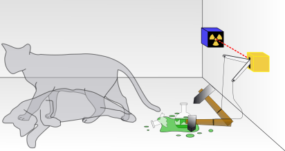
Schrodinger’s cat experiment: the cat, tied to the fate of a quantum particle, is simultaneously alive and dead until “measured.” Image by Dhatfield.
The idea is simply this: by putting the cat in the box which is linked to the radioactive atoms, we are entangling the cat with the atoms. We may write the quantum state of the combined cat and box system as follows.

This goes back to the question: “what is a measurement, and who does the measuring?” If we consider the cat part of the quantum system, then it is simultaneously living and dead in the box until we open the box and see the result. Or does the cat count as a measuring device? Or is it the radioactive detector that detects the radioactive decay? These questions get right to the heart of the puzzle: how do we interpret quantum physics? This is a puzzle that we are still not sure how to solve.
We do, however, know and understand a lot more than I can cover in this post! In the next post in this series, we will take a look at the issue of entanglement and relativity discussed above, and see how to resolve the seeming conflict between them. In a future post, we will address the issue of “hidden variables” that EPR introduced, and the answer will surprise us! I also hope to discuss how physicists today generate entangled quantum particles in the laboratory, and also discuss some of the possible applications of quantum entanglement, such as quantum cryptography and quantum computing. I will also try and discuss going “beyond Copenhagen”: different interpretations of quantum physics that avoid the measurement problem and wavefunction collapse that we have discussed.
As you can see, we still have quite a lot of physics to untangle!
****************************
† If you want to learn a little more about quantum spin, please see my article on experiments with neutron spin.
¹ You may have noticed that there is a minus sign in the equation for the electron and positron together, where we had a plus sign for our double quarter. When one rigorously calculates the quantum state of the electron positron combination, that minus sign is necessary for the total spin to be zero. It doesn’t affect our argument here; I only include it so that physicists don’t yell at me.
² I borrowed some wording here from my recently-published Singular Optics textbook, as I didn’t think I could improve upon it.
³ Einstein, Podolsky and Rosen, “Can quantum-mechanical description of physical reality be considered complete?” Phys. Rev. 47 (1935), 777–780.
4 Schrödinger, “Die gegenwärtige Situation in der Quantenmechanik (The present situation in quantum mechanics)”. Naturwissenschaften. 23 (1935), 807–812.


Part 3 excelent ! Thank you indeed.
A very good post. I await further explanation of entanglement and relativity. I would like to prepare an “Enrichment Lecture” for cruise ship passengers on quantum entanglement. Any comments?
Thank you for this enjoyable and informative series. I came across Part 3 via Flipboard, and, learning there were Parts 1 and 2, I read them then read Part 3. Wonderful explanations.
We can say that there is a DNA associated with each subatomic particle which determines the spin state
Great explanation that includes both ideas.😎✨
I may have missed it or have not understood, but how do we “know” that a particle exists in superposition instead of on a predetermined path?
This is, in essence, how we interpret the wave properties of particles. The fact that we get wave interference in systems like Young’s double slit experiment indicates that we have interference of the waves emanating from the two slits.
In that experiment, why the wavefunction “collapses” when hitting the final screen and not when hitting the double slits panel?
The way I’ve always interpreted it: lots of electrons *do* hit the slit screen and “collapse” and are absorbed or scattered by it; those electrons do not make it through the slits. In essence, the only electrons that one sees are those that successfully made it through the slits and didn’t interact with the slit screen.
This may be the single best mental model of entanglement that I’ve ever read. Thank you!
You’re welcome!
BRILLIANT!! BRILLIANT!! BRILLIANT!!
Continue the good work.
I don’t get this assertion: “However, because of angular momentum conservation, the positron must have instantly collapsed into the spin-down state.” Could you please point me were I can read about why the momentum of both particles would still be linked the instant after the original particle decays? Here is my problem: at the instant of the decay, the system transitions from one pion to the pair electron/positron. Momentum of that system is conserved during the transition. Right after that instant the system is the universe. Momentum is still conserved, in the universe system. Why would there be any unique relationship between electron and positron, somehow different than their multiple relationships to all the other particles in the universe?
What is quantum entanglement you can see from the point of physics derived from the principle of probability?
http://readgur.com/doc/3558406/space-time–principles-physics-of-chances
The book is removed to the site:
Click to access principles.pdf