Update: fixed a mistake in my numbers for telescope resolution, which I had worse by a factor of 10.

Science is in general intended to be a serious business, but every once in a while one comes across some serious research that also ends up being incredibly funny. Sometimes this is deliberate humor on the part of the scientists — like the time that Athanasius Diedrich Wackerbarth destroyed Charles Piazzi Smyth’s “pyramid power” series of pseudoscientific articles — but sometimes the humor just falls out naturally in the course of a scientific debate.

One of my favorite of the latter cases is the controversy that arose in the 1950s surrounding the functioning of a new type of interferometer introduced by Robert Hanbury Brown and Richard Q. Twiss. Describing this controversy is an excellent opportunity to introduce the science of what is known as intensity interferometry and leads up to what is to me a hilarious punchline.

To begin, we need to look at the limitations of conventional imaging systems, and how Albert A. Michelson found a method to work around those limitations in the 1890s.

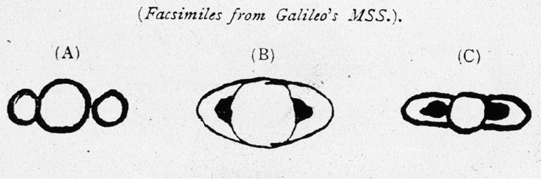
For centuries, humans have used telescopes to directly image stellar objects. This arguably started with Galileo in 1609 when he used one of the first refracting telescopes to observe that the surface of the moon is not smooth; within a year, he had observed the four largest moons of Jupiter as well as the rings of Saturn, and sketched them as shown below. As the orientation of Saturn changed, the rings seemed to disappear, which made Galileo remark, in a very mythological callback, “Had Saturn devoured his children?“

Telescopes are fundamentally limited in their resolution by the size of the telescope aperture, i.e. the opening of the telescope that collects light. Galileo’s original telescope had an aperture of only 2 inches, and its resolution was understandably poor. In fact, one can determine that the angular resolution of a telescope — the smallest angular separation of objects that can be distinguished by the telescope — is given by the formula 1.22*(wavelength)/D, where D is the aperture size and (wavelength) is the wavelength of light. For example, if we assume we are imaging objects using visible light, which has a wavelength of around 500 nanometers, and assume a telescope aperture of 3 meters, we find that the angular resolution is about 0.04 arcseconds. As the inclusion of the wavelength in the formula suggests, the resolution limit of a telescope is a consequence of the wave nature of light.

An arcsecond is 1/3600th of a degree, so it appears that our telescope has great resolution — until you look at the angular sizes of objects in the sky. At their closest points of approach, Mars has an angular size of 25.1 arcseconds and Uranus has an angular size of 4.1 arcseconds, making them resolvable but with very little detail. The largest telescope on Earth has a diameter of 11.8 meters, which only gives an angular resolution improvement to about 0.01 arcseconds. It is extremely impractical, if not nearly impossible, to make actual physical telescopes with apertures larger than this.

If we start to look at objects outside our solar system, we find that the angular resolution of an ordinary telescope is simply insufficient to do any significant imaging. Proxima Centauri, the closest star to the Earth past the sun, has an angular size of 0.001 arcseconds. Curiously, we can do a little better with Betelgeuse, which has an angular size of 0.06 arcseconds due to its utterly massive size even though it is farther away. But by the late 1800s, it was clear that most stars outside of the solar system will only appear as points of light in a conventional telescope.¹ But physicists are curious people, and want to know more about these stars, such as the very basic question: how big are they?

Into this situation came the brilliant Albert A. Michelson, an American physicist who had already become famous for his extremely precise interferometers and their use in, among other things, attempts to measure variations in the speed of light — the Michelson-Morley experiment. Interferometry is the use of wave interference to measure properties of the objects that emit the waves or the waves themselves. A classic example is called the Michelson interferometer, which splits a light wave into two parts, sends them along paths of different lengths, and then brings them back together to interfere. A simple illustration of this interferometer is shown below.

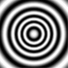
Light from the source S is split into two beams at the partially reflecting mirror M₀ and each beam reflects off of a mirror and is then recombined at a screen B. If there is a distance d between the paths, then one will see interference fringes — bright and dark rings of light — at the screen, as illustrated below.

The power of interferometry is that it is extremely sensitive to small changes — if the path difference in the Michelson interferometer is changed on the scale of a wavelength, the fringe pattern will change. Thus, by measuring fringes, one can measure extremely small differences in a light wave or properties of its source. This is basically how Michelson and Morley looked for variations in the speed of light — they looked for changes in the fringe positions when the interferometer was oriented in different directions with respect to the motion of the Earth around the sun. Beyond this, Michelson realized that interferometry could potentially be used to extract information about stellar objects that was unobtainable with the existing technology of the day.

We have noted that the resolution of a telescope is restricted by the inherent wave nature of light. In short, waves tend to spread out as they propagate, and this puts a fundamental limit on how sharp an image can be. Using a larger aperture allows waves to be focused “tighter,” producing a sharper image, but as we have noted it was definitely impractical in Michelson’s time to create significantly large telescopes (and it still is).

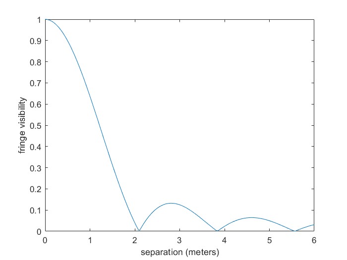
Instead of collecting light over an entire telescope aperture, however, Michelson imagined collecting light from only two spatially separated points within the aperture. The light from these points could be brought together and interfered, and Michelson showed that the visibility of the interference fringes — the contrast between the bright and dark rings — directly depends on the angular size of the light source. The formula indicates that the fringes will disappear entirely when the separation of the points is 1.21*(wavelength)/(angular size). If one measures the visibility of the interference fringes as a function of the separation of the points, and determines the separation at which the visibility vanishes, one can directly determine the angular size of the source. A simulation of what one would see for the star Betelgeuse is shown below, which also gives an idea of the separation needed to achieve this result. Note that the zero of fringe visibility is only about 2 meters, which means that the size of Betelgeuse can be determined with a quite small separation!

In other words, instead of trying to capture an image of the object directly, Michelson suggested using interferometry to deduce the size of the object. Because of the sensitivity of interferometry, the interference experiment would be able to accurately measure this size beyond what a comparable telescope could do via direct imaging.

Incidentally, if you want to know why the fringe visibility depends on the angular size of the source… well, that brings us into some optical coherence theory and a significant amount of math, so we’ll skip the details here.

Michelson first proposed this idea in two papers in 1890, and imagined modifying an ordinary telescope to perform the experiment.² But why use a telescope at all, when large telescopes are difficult to construct and not actually needed? All that is needed is to collect light from two spatially separated points, ideally using a device where the separation can be changed to make a figure like the one above. In 1921, Michelson and collaborator F.G. Pease introduced³ a new device that is now known as the Michelson stellar interferometer; their original illustration of the device is shown below.

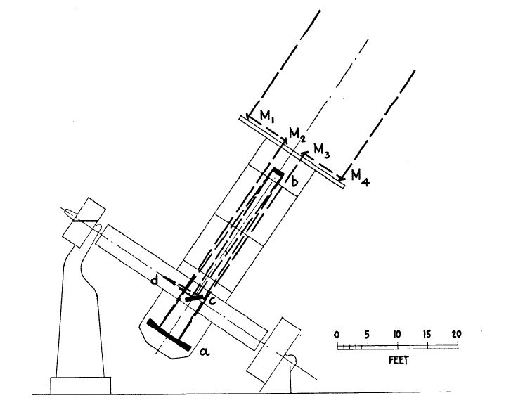
The device is pointed at the stellar object of interest, light from two separated points is collected at mirrors M₁ and M₂ and that light is combined and focused at a point d. The two outer mirrors can be moved to allow the interference fringes to be observed for various separation distances, allowing the magic zero visibility point to be found.

Michelson and Pease applied this result to the star α-Orionis, which is the technical name for Betelgeuse. They found the size to be 0.047 arcseconds, comparable to the modern estimate given above. An “exact” value of the size of the star is not known, because there are evidently variations in the star’s behavior over time and the Michelson calculation depends on making an assumption of the intensity distributed over the star. This is highlighted by Michelson and Pease’s version of my theoretical calculation, shown below.

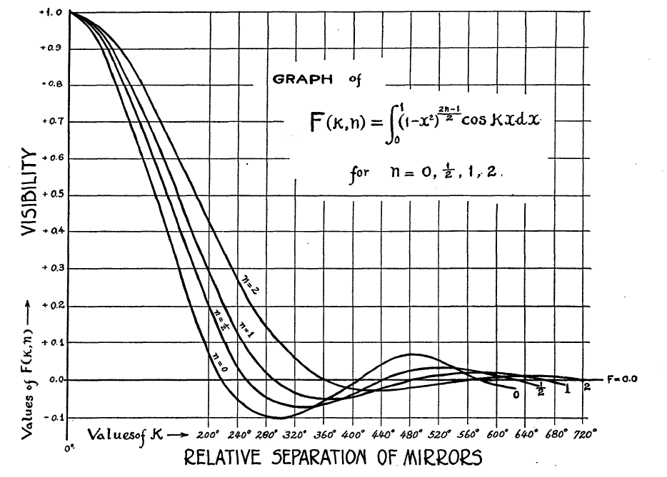
Since they didn’t know what the brightness distribution of the star is — is it uniform brightness, or brighter in the center? — they plotted theoretical calculations for a number of scenarios. Most people assume today that stars are effectively of uniform brightness.

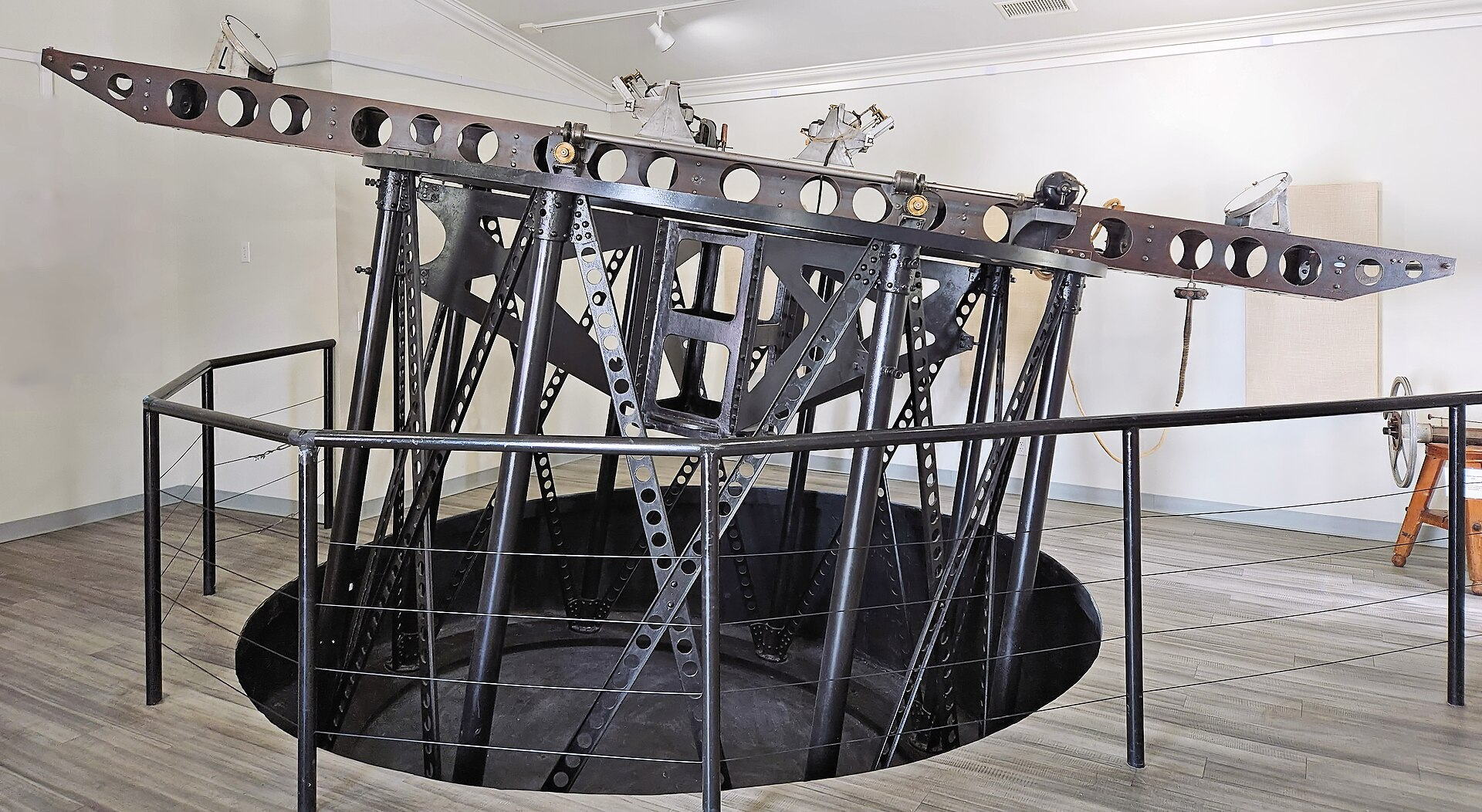
Michelson’s interferometer was installed at Mount Wilson Observatory, and I believe the photograph below is an image of the original interferometer, now on display at the observatory. The separation between the outside mirrors was up to 6 meters.

Why did it take so long from Michelson’s first introduction of the concept of the stellar interferometer to one actually being tested? It appears that in part it was because nobody was sure that it would work. In principle the idea seemed fine, but in practice the light from the cosmos would first pass through turbulence in the atmosphere that would distort the waves and potentially ruin the wave interference. The first test of the interferometer showed, however, that turbulence did not significantly affect the results.

Michelson’s interferometer was a great leap forward, allowing the sizes of stellar objects to be measured for the first time. However, it was itself limited by practical considerations. Because the device depends on wave interference, light from the two arms of the interferometer has to be directed by the mirrors to the interference point, and this becomes increasingly difficult the larger the device gets. Furthermore, the entire device must be rigid and must be attached to a telescope so that it can be rotated to view different stars — one can imagine that it becomes impractical to have such a device when the mirrors are, say, 20 meters apart. To go much further, a modified or completely different approach would be needed.

Let us fast forward a decade to the early 1930s. Karl Jansky, working at Bell Telephone Laboratories, set up a system to measure the direction of short-wave radio signals and, presumably, their origin. It was well-known that there is a constant “hum” of short-wave radio static on Earth, and Jansky was attempting to determine its origin. In his first publication in 1932, Jansky noted⁴ that short-wave static seemed to have 3 sources: nearby thunderstorms, distant thunderstorms, and “unknown.”

The unknown radio sources were baffling, and seemed to change position periodically on a 24 hour cycle. An astronomer colleague of Jansky pointed out that this suggested that the source of the radio waves was outside of our solar system, effectively fixed in position but seeming to change direction because of the 24 hour rotation of the Earth. This was the discovery of cosmic radio sources, and Jansky announced his discovery in July of 1933.⁵ In particular, Jansky had discovered a tremendous source of radio waves emanating from the center of the Milky Way galaxy. Soon, researchers would find that the sky is filled with radio sources.

Jansky’s discovery received a lot of attention, though it would take a number of years before astronomers actually began to study these mysterious cosmic sources of radiation. It was a tremendous and exciting time: the existence of previously unknown sources of radio waves allowed for new insights into the physics and nature of our universe. They were, however, a genuine mystery: the radio sources did not seem to coincide with sources of visible light, i.e. stars, and nobody had any idea what they might be. Furthermore, attempts had been made to try to measure the angular size of these sources using tricks that amounted to a Michelson-type stellar interferometer, but it was found that the interferometer arm separation available was not sufficient to determine the size of the radio sources. The biggest issue is that the wavelength of the radio waves of interest was on the order of a meter, some 5 orders of magnitude larger than the wavelength of light! This meant that the separation of the interferometer arms needed to be somewhere on the order of tens or hundreds of kilometers to achieve the same resolution as light. Again, a new technique was needed if answers were to be found.

The new technique was introduced in 1952 in R. Hanbury Brown, R.C. Jennison and M.K. Das Gupta, in a paper⁶ titled “Apparent angular sizes of discrete radio sources.” I share their original diagram of the system below.

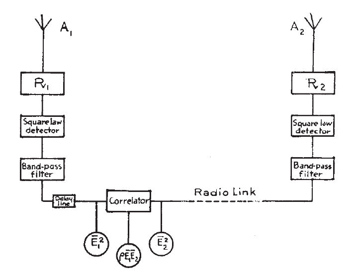
There are two receiving antennas, representing the two arms of the interferometer, that collect the radio signals. These signals are converted with electronics and then brought together at a correlator, which effectively “interferes” the signals together analogous to a Michelson interferometer.

The key change from earlier systems is the use of “square law detectors.” An ordinary antenna converts a radio wave into an electrical current proportional to the wave amplitude. A square law detector instead converts the incoming wave amplitude current into an output wave intensity current — the output current is proportional to the wave amplitude squared. In a Michelson interferometer, the wave amplitudes are interfered together to extract information, but in this new interferometer, the wave intensities are interfered together to get the information.

Why do this at all? The current produced by a a radio signal amplitude has a very high frequency of oscillation and it gets strongly attenuated in an wire used to transmit it, limiting the range over which the antennas can be separated. Ever more important, however, is that the signal amplitude has a very fast oscillating phase — the frequency of oscillation of the radio wave — and the further apart the antenna are spaced, the more difficult it becomes to avoid phase errors that ruin the measurement. The intensity interferometer avoids both of these problems — the intensity does not possess the rapidly-oscillating phase, which means that it can be transmitted with small error and small attenuation over extremely long distances — even by converting it into another radio signal and broadcasting it to the correlator! With this approach, the two antennas could be easily separated by distances of kilometers, and the size of radio sources could be determined with accuracy far exceeding anything previously possible.

The researchers tested their system on the radio galaxy Cygnus A, using multiple measurements with baselines that ranged from 300 m to 15 km. By orienting their antennas along different lines, they were able to not only measure the size of the source but also measure the size along different axes. They found that Cygnus A has a size of roughly 35 arcseconds to 2 minutes 10 seconds of arc. This dramatic asymmetry is understood by looking at a modern, high-resolution, radio image of Cygnus:

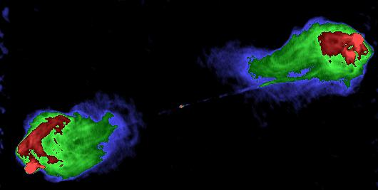
What is actually happening in Cygnus A is that a supermassive black hole at the center of the galaxy is producing two jets of higher energy materials. These jets then collide with intergalactic gas, and radio frequency radiation is produced in the collision. As I said, radio astronomy leads to many novel insights about the universe!

The idea that one could do interferometry using wave intensity rather than wave amplitude was a new one, and in 1954 Hanbury Brown and Richard Q. Twiss (HBT) published a paper⁷ outlining in detail the theory of the technique, showing the conditions under which it could work. It appears that this paper is the one that captured the most attention, and the interference of intensities became known as the Hanbury Brown Twiss effect. (Many people at first glance assume that there are three authors, but Hanbury Brown is one name.)

This is the point where things got controversial. Hanbury Brown and Twiss, fresh off the success of using their new interferometer for radio waves, wondered if they might be able to use intensity interferometry for light waves. We have noted that the ordinary Michelson stellar interferometer, which redirects light waves using mirrors to a point of mutual interference, is limited to a mirror separation of around 10 meters. If one instead measures light intensity at two points, that intensity can be conveyed over extremely long distances via wires — think kilometers — and if intensity interferometry works, the angular size resolution of the interferometer could be improved by a factor of 10 or more. Hanbury Brown and Twiss tested this idea in a laboratory experiment and published⁸ their results in 1956 in a paper titled, “Correlation between photons in two coherent beams of light.” This experimental setup is reproduced from their paper below.

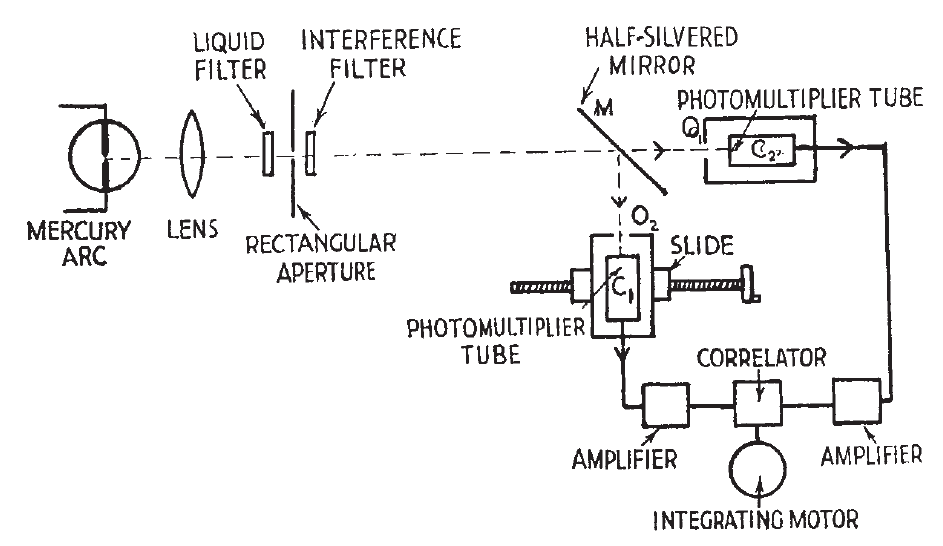
Without going into too much detail, the idea is as follows. The light from a mercury arc lamp is focused onto a rectangular aperture to form a source of light of finite size. The detectors are two photomultiplier tubes that detect the light intensity. To simulate the idea of two spatially separated detectors, the beam of light is divided in two at a half-silvered mirror, and one of the photomultiplier tubes is able to be moved horizontally, to effectively act as a transverse separation of the detectors. Then the intensity signals from the two tubes are brought together in a correlator and the correlations are measured, as in the radio frequency case.

Hanbury Brown and Twiss reported that they were actually able to see correlations. When the separation of the two tubes was effectively zero, they saw large correlations, and when the separation was large, they saw no correlations.

This would seem at a glance to be a straightforward experimental confirmation of the Hanbury Brown Twiss effect with light, but objections were immediately raised on the physical differences between light waves and radio waves and the nature of the detectors used in each case. Though all electromagnetic waves have quantum wave-particle duality, the long wavelength of radio waves makes them act almost entirely wavelike. The square law detectors used to measure the intensity therefore make an almost directly measurement of the wave intensity of the radio waves.

Photons, however, have a wavelength orders of magnitude smaller and they act much more particle-like, and a photomultiplier tube used to detect light intensity takes advantage of the photoelectric effect, in which individual light photons liberate individual electrons on a metal surface, creating a current. These electrons are then “multiplied” by accelerating them with a high voltage, which on collision with another metal surface causes more electrons to be liberated.

So a photomultiplier tube basically counts photons arriving at the detector, and not wave intensity. Photon count should be roughly proportional to wave intensity, but because photons are particles, their energy arrives in discrete bits and that random arrival of bits of energy shows up as noise in the system, usually called “shot noise.” In this case, shot noise is purely a quantum mechanical effect.

Skeptics of Hanbury Brown and Twiss’ results argued that shot noise would prevent any meaningful correlations to be detected in intensity interferometry using light, making the technique useless. In particular, Brannen and Ferguson⁹ tested HBT’s results and concluded that intensity correlations did not exist, and they quoted earlier null results by Adam, Janossy and Varga¹⁰ to bolster their argument.

Here is where the phrase “a little knowledge is a dangerous thing” becomes relevant. The whole idea of looking at intensity correlations for photons was incredibly new, and many researchers did not fully understand the subtlety of the phenomenon. In particular, there is a parameter now known as the degeneracy parameter that characterizes whether intensity fluctuations are dominated by the (desired) wave fluctuations of light or the (not desired) shot noise. This parameter, even for thermal sources over a reasonable range of temperatures for visible light, can vary over a range of 40 orders of magnitude, with a peak value of around 10 in that range. Considering that degeneracy parameter must be comparable to or greater than one to see the desired HBT effect, it was very easy for researchers not fully versed in the theory to completely miss the mark.

This is what Hanbury Brown and Twiss pointed out in a follow-up 1956 paper¹¹ “The question of correlation between photons in coherent light rays.” In the paper, they ran the numbers and estimated how long each experiment — theirs, Brannen and Ferguson and Adam, Janossy and Varga — would need to collect data in order to produce a measurable intensity correlation.

The experiment of Hanbury Brown and Twiss required 5 minutes of data collection to produce a signal. The experiment of Brannen and Ferguson would require 1,000 years to produce a signal. And what about Adam, Janossy and Varga? Their experiment would require 1,000,000,000,000 years, or 10¹² years. The age of the entire universe is estimated to be around 10¹⁰ years.

This is the punchline that I alluded to at the beginning of this very lengthy post! The first time I read these numbers provided by HBT, I laughed a lot. Maybe it’s just funny to a physicist, but being that wrong about something is hopefully pretty hilarious to anyone.

I should note that this is not intended to be a laugh at the expense of the researchers in question. Science is challenging and a researcher working on the cutting edge of research is bound to make mistakes or draw incorrect conclusions, even if they are extremely diligent — it comes with the territory. In every good scientific debate, there is going to be a right answer and a wrong answer, and science is enriched by the discussion from both sides.¹²

The Hanbury Brown Twiss effect is now fully accepted by the scientific community, and it is an important tool in both theoretical and practical optics endeavors. HBT went on in November of 1956 to publish their first astronomical test¹³ of their intensity interferometer for light in a measurement of the angular size of the star Sirius. Using a maximum baseline of 9.2 meters, they measured the angular diameter of Sirius to be 0.0063 arcseconds. Recalling that Michelson’s first achievement with his stellar interferometer was the measurement of Betelgeuse at a size of 0.047 arcseconds, we can see how significantly the HBT interferometer advanced measurement sensitivity.

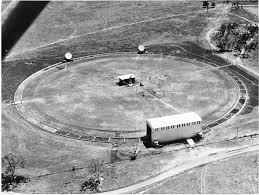
Hanbury Brown went on to design a Stellar Intensity Interferometer near the town of Narrabri in New South Wales that operated from 1963 to 1974. It had two detectors that could be moved along a large circular track to change the baseline from 10 meters up to 188 meters, further improving the sensitivity of the system.

Beyond being a very cool and practical technique (with an unintentionally funny punchline), the Hanbury Brown Twiss effect started a new discussion and understanding of the wave-particle nature of light that continues to this day. But that is a topic for another post, as this one has gone on for quite some time!

*************************************************

1. You might wonder what the point is of having larger telescopes if we can’t really produce good images of individual stars. Well, the point is that we are interested in measuring the location of the stars and their brightness. One thing that a larger telescope aperture does for us is allows us to collect a lot more light, which means we can see objects in the sky that are too dim to see with the naked eye, like ancient distant galaxies.
2. A.A. Michelson, “Measurement by light waves,” American Journal of Science, issue 230 (1890), 115-121, and A.A. Michelson, “On the Application of Interference Methods to Astronomical Measurements,” Phil. Mag. S. 5 V. 30 (1890), 1-21.
3. A.A. Michelson and F.G Pease, “Measurement of the diameter of α-Orionis with the interferometer,” Astrophysical Journal, 53 (1921), 249-259.
4. K.C. Jansky, “Directional studies of atmospherics at high frequencies,” Proc. IRE 20 (1932), 1920-1932.
5. K. Jansky, “Radio Waves from Outside the Solar System,” Nature 132 (1933), 66.
6. R. Hanbury Brown, R.C. Jennison and M.K. Das Gupta, “Apparent angular sizes of discrete radio sources,” Nature 170 (1952), 1061-1063.
7. R.H. Brown and R.Q. Twiss, “A new type of interferometer for use in radio astronomy,” Phil. Mag. 45 (1954), 663–682.
8. R.H. Brown and R.Q. Twiss, “Correlation between Photons in two Coherent Beams of Light,” Nature 177 (1956), 27–29. 
9. E. Brannen and H. Ferguson, “The Question of Correlation between Photons in Coherent Light Rays,” Nature 178 (1956), 481–482.
10. Adam, Janossy and Varga, Acta Physica Hungarica 4 (1955), 301.
11. R.H. Brown and R.Q. Twiss, “The Question of Correlation between Photons in Coherent Light Rays,” Nature 178 (1956), 1447–1448.
12. I should note that this doesn’t include artificial “debates” over things that have long been settled, like “vaccines are good,” “the Earth is round,” “climate change is real,” and “the moon landings happened.”
13. R.H. Brown and R.Q. Twiss, “Test of a New Type of Stellar Interferometer on Sirius. Nature 178 (1956), 1046–1048.