Preparing to write the final section for the second edition of my Singular Optics textbook that happens to be on, you guessed it, optical skyrmions! I thought I would try writing a non-technical explanation first to straighten out all the concepts in my head.

One of the big evolutions in the field of optical physics over the past twenty years has been the introduction of the mathematics of topology into almost all aspects. This has led to a lot of interesting phenomena in optical wavefields themselves such as optical vortices, optical knots and optical Möbius strips. (What is “topology?” We will come back to that in a moment.)

In the past decade, a lot of research has focused on a different sort of topological feature that can arise in optical wavefields, known as a skyrmion. The name comes from Tony Skyrme, who first introduced this topological feature in a paper¹ in 1961 as a possible model of a nucleon. Optical physicists, having drawn lots of inspiration from topology previously, began investigating the possibility of having skyrmions in optical wavefields in 2012 and there has been an intense amount of research since then.

So what is a skyrmion, what is an optical skyrmion, and for that matter, what is topology? Settle in for a lengthy post as I try to walk through all of these concepts! The discussion will be non-mathematical and as non-technical as I can get, but we will have a lot of ground to cover.

Let us start by trying to answer the question: What is topology? Borrowing from Wikipedia, topology is “the branch of mathematics concerned with the properties of a geometric object that are preserved under continuous deformations, such as stretching, twisting, crumpling, and bending; that is, without closing holes, opening holes, tearing, gluing, or passing through itself.”

That is already a lot of words, but we can use a classic example as an illustration. Let us imagine that we fashion a coffee cup out of clay; if we are allowed to stretch and deform the clay, we can with some effort fashion it into a donut:

It turns out that the indentation in the coffee cup where the coffee goes isn’t really a fundamental part of the structure, but the hole is. Thus we can say that a coffee cup is “topologically equivalent” to a donut. A coffee cup is not topologically equivalent to a sphere because I cannot make a cup into a sphere without sealing the hole, or a sphere into a cup without opening a hole. This can all sound very fuzzy, but rest assured it has a very precise definition in mathematics. Opening or closing a hole does not count as a “continuous deformation.”

These topological properties can often be quantified in what are known as topological invariants: numbers associated with a structure that don’t change under the allowed types of deformations. A classic example is the Euler characteristic, which is commonly used to characterize the structure of polyhedra. Consider, for example, the following familiar polyhedra:

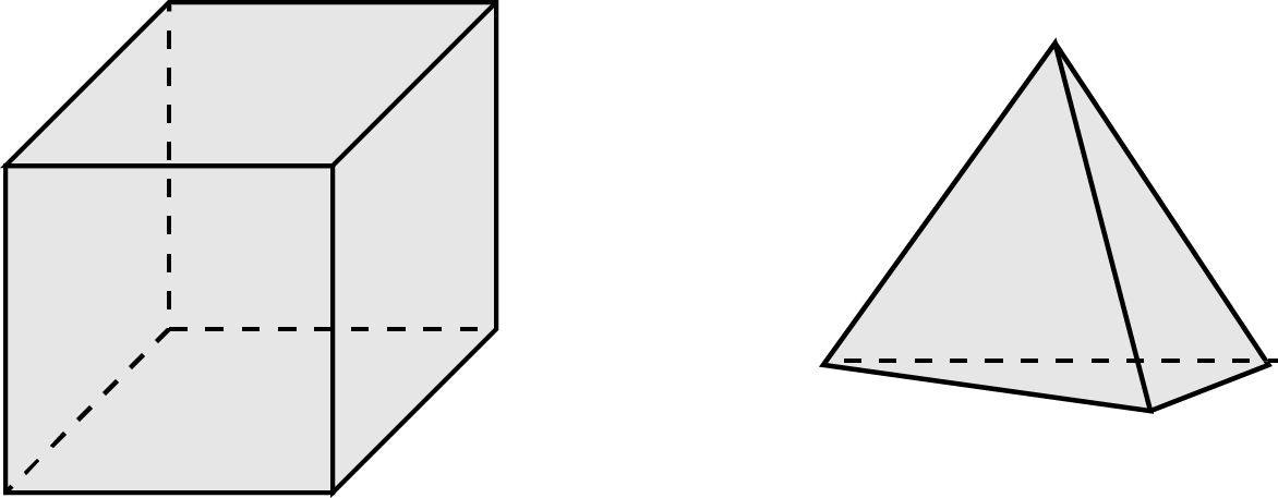
(I have only drawn two of the many familiar polyhedra for my own sanity.)

Now count the number of vertices V, edges E and faces F of each of these, and calculate the quantity

N = V – E + F .

You will find for the cube that N = 8-12+6 = 2 and for the tetrahedron N = 4 – 6+4 = 2. If you use any of the Platonic solids, like a dodecahedron, you will find that all of them have N = 2! Now consider the following two modifications:

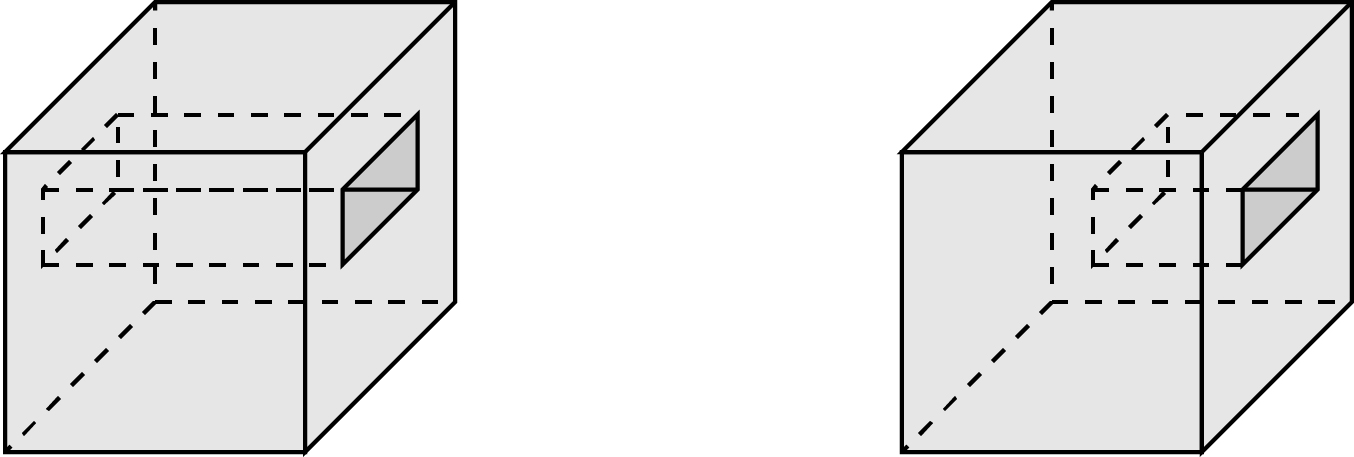
For the cube on the left, with a tunnel in it, we now have N = 16-24+8 = 0. Why is the number of faces 8? Our initial argument didn’t include a simple rule to quantify faces with holes in them, so we must clarify our arguments. The two holes in principle can be expanded right to the edges of the cube to remove the two faces with holes in them entirely, thus reducing the number of faces by 2. Another way to think of it: slightly indent each of the faces with holes in them, creating four new edges but also four new faces, making the net contribution of each of these sides zero.

For the cube on the right, we have N = 16-24+6 = 2 again: the one face “removed” by the hole is countered by the new face inside the hole. Again we have a situation where a “hole” changes the fundamental property of the structure, but a “dent” does not.

One more quick illustration of this: suppose we make a dent by poking one face of the cube with our finger, giving something like this.

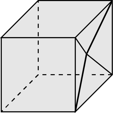
One face has become four, so we’ve added three faces; however, we’ve also added one vertex and four edges, so the total for N remains 2!

There are other shapes with other distinct N values, and the concept of the Euler characteristic can be generalized to smooth shapes, so that a sphere has N = 2 and a torus (donut) has N = 0.

This gives you an idea of how there are some features of a geometrical structure that are resistant to deformations and can be quantified. These concepts may seem abstract and not very useful, but topology turns out to be a perfect example of how “useless” mathematical concepts can become fundamentally important in physics!

At first glance, it might seem that optical waves are very far removed from topology. The topology we’ve considered so far is for solid, or at least well-defined, objects, where waves are by their nature somewhat amorphous. Waves can diffract, interfere, and generally spread out or get distorted when they encounter obstacles. But waves satisfy well-defined physical and mathematical laws themselves, and those laws provide restrictions on what waves can and cannot do. From those restrictions, we can find well-defined topological features of waves.

Let’s look at some relevant wave basics, which will then take us to optical vortices, the most well-known topological structures in wavefields. (I will reiterate and reuse information from an older post on singular optics.)

We begin by visualizing monochromatic (single frequency of oscillation) waves on a string, as might be generated by waving the end of the string up and down in a regular manner. A snapshot of the string at an instant of time would look something like this, where the arrow indicates the overall direction of motion:

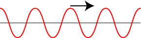
Because the “waving” of the string repeats itself regularly, we can characterize its state by an angle between 0 and 360°, with 0 representing the situation when the wave is at its peak:

This angle is what we refer to as the phase of the wave. At the wave is at its highest; at the wave is at its lowest. At the wave has no height but is moving upward; at the wave also has no height but is moving downward. For future reference, we refer to those regions for which as the wavefronts of the wave.

We can also define a phase for an optical wave in three-dimensional space.  The simplest is a wave where the wavefronts are equally spaced planes in 3-D space; such a wave is known as a plane wave (here shown moving to the left):

Let us view the wavefronts as the “structure” of the wave, and in this case the wavefronts are stacked parallel on each other, like layers of a cake or floors of a building. We can then ask: are there other ways that the wavefronts of a wave can be arranged?

Let us look at the stack of wavefronts, now arranged vertically, and on each wavefront we start from the center and slice a line out to the edge. We then pull the back edge of each cut downward to join with the front edge of the previous wavefront. The result looks something like what is shown below.

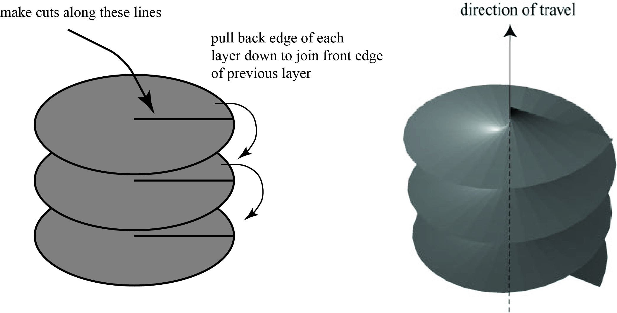
What you end up with is a set of wavefronts joined together to form what looks like a screw, and in fact the technical name of this structure is “screw dislocation.” Note that I had to again make cuts in order to construct this screw dislocation from a collection of planar wavefronts, which is the sort of thing we’re not allowed to do in topology: we can say that this screw wave is topologically distinct from the planar wave. Even though we have introduced “no cuts” as a mathematical rule, the physics of waves prevents such cuts from ever arising in a monochromatic wave, so this topological structure is preserved even if we distort the wave.

Incidentally, you have seen such structures in real life all the time, though you may not have realized it! A multilevel parking deck, with ramps smoothly connecting the different floors, acts like a screw dislocation. It is topologically distinct from a normal office building with separate non-interconnecting floors that acts more like a plane wave.

Beams that have a screw-like twist in their wavefronts are typically called vortex beams, because the wavefronts circle around the central axis like water swirling around a drain. The identification of vortex structures in wavefields was first done by Nye and Berry² in 1974, launching an entirely new field of topological studies of light.

Can we quantify this vortex structure? Let us suppose we look at the phase of the wave in a cross-section perpendicular to the direction the wave is going; this is exactly the sort of thing a detector would measure. There is an entire class of vortex beams known as Laguerre-Gauss beams, and we show the intensity and phase of three examples below.

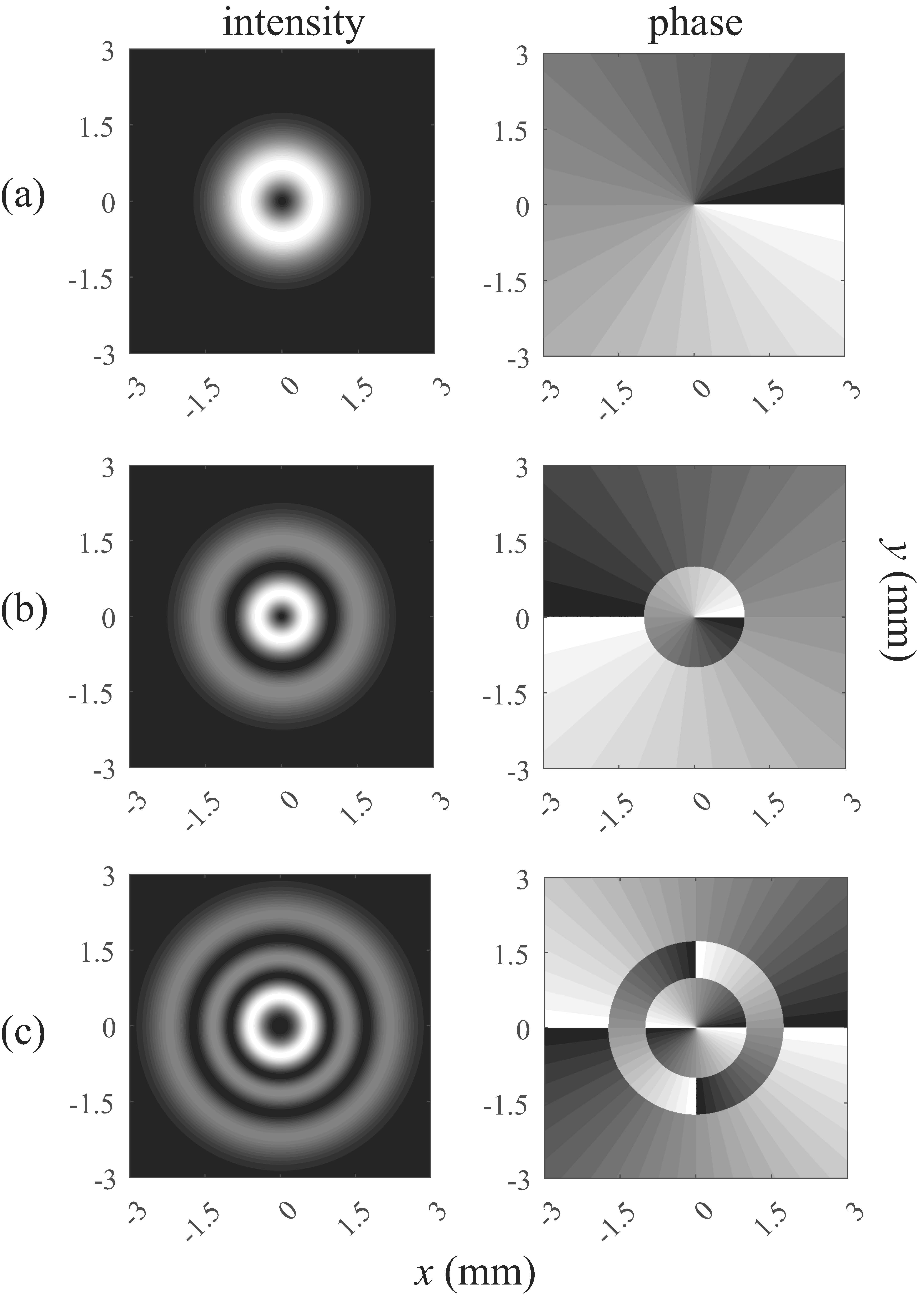
The cross-sectional brightness (or intensity of the beams are the left column, and the phase is on the right. Black represents zero degrees and white represents 360 degrees. Look at the way the colors evolve as one travels counterclockwise around the center axis of the beam. In (a), the phase increases continuously from 0 to 360 degrees; remember that mathematically 360 degrees is the same as zero! In (b), the phase decreases from 360 degrees to zero, and in (c) the phase increases twice from 0 to 360 degrees.

It turns out that the phase will always increase or decrease by an integer multiple of 360 degrees when going around the central axis of a vortex; this integer multiple is called the topological charge of the vortex. In (a) the charge t = 1, in (b) the charge t = -1, and in (c) the charge t = 2. The topological charge is the topological invariant of a vortex structure, like the Euler characteristic is the topological invariant of polyhedra. Waves with different topological charges have distinct topological structures.

So there are two very significant properties of vortex beams: they have an integer topological charge and that topological charge is resistant to perturbations of the wavefield, just like a donut stays a donut even if you smush it and deform it. These two properties together have made vortex beams an intense area of study for free space optical communication. When light propagates through the atmosphere over long distances, atmospheric turbulence tends to distort the signal, leading to errors in communication. Because a vortex structure possesses some robustness, using the vortex structure itself as the information carrier has potential to make long distance communication more reliable. Furthermore, it is possible to send information simultaneously through different vortex beams and separate them at a detector, allowing more information to potentially be sent along a single channel.

A vortex is in fact a singularity of a wavefield; if you look at the cross-section plots above, you will see that there is a zero of intensity at the center of the beam and all the phase values converge at that point. The phase is undefined, or singular, at the beam center; the study of wavefield singularities has therefore become the subfield of optics known as singular optics.

Most of singular optics has focused on actual wavefield singularities, but as we have seen in the Euler characteristic there are topological quantities and structures that are protected without being singular. This observation brings us, at last, to the concept of an optical skyrmion.

It is probably best at this point to just show you what such a skyrmion looks like and then explain what you’re looking at! This is a plot of a single isolated optical skyrmion:

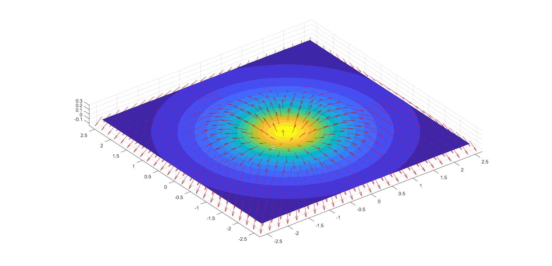
You will first note that this is a two-dimensional plot, like the cross-section of the vortex phases shown earlier. A skyrmion studied in two-dimensional systems is officially labeled as a “baby skyrmion,” but these are the ones that are relevant for optics.

At each point in the two dimensional plot, there is an arrow. These arrows represent a three-dimensional directional field in the two-dimensional space. To put it another way, at each point in the two-dimensional plane, we have an arrow pointing in a definite three-dimensional direction. Every arrow is the same length; the only difference between them is their directions. The colored plot underlying the arrows shows the length of the arrow in the vertical direction.

Now look at the actual directions of the arrows in the plot. In the center, the arrows point directly up; on the periphery of the plot, the arrows point down. You can also see that the arrows largely point radially outward from the center. A little inspection should convince you that every three-dimensional direction appears in this figure, or that the arrows in the plane cover every possible three-dimensional direction, and cover them exactly once.

This structure — a two-dimensional vector field that entirely covers every three-dimensional direction — is the topological structure that constitutes a skyrmion (or more precisely, a baby skyrmion). Because the arrows cover every three-dimensional direction exactly once, the skyrmion number equals 1. The skyrmion number is the topological invariant for the skyrmion, like the Euler number or the topological charge. It can be shown — though it is way beyond our goals for this post — that this skyrmion number is always an integer value. Like topological charge, it can be positive, negative or zero. How can it be negative? The rigorous definition of the skyrmion number depends not only on the number of times that the field covers every three-dimensional direction but also the way it does so, analogous to how the topological charge can be positive or negative depending on the way the phase changes around the vortex axis.

It is worth noting that there is nothing “singular” about this skyrmion configuration: the arrow direction is well-defined at every point. It is a topological characteristic of a field that is not connected to a singularity.

Outside of particle physics, skyrmions really gained traction in magnetic systems. The first paper appeared³ in the journal Science in 2009 and from there magnetic skyrmions became a new area of research with the potential to use them as information carriers in magnetic data storage, much like vortices are considered as data carriers in optics. With this in mind, it was likely inevitable that researchers would turn to finding skyrmions in light fields.

The first question to ask: what represents the directional field in the optical case? In magnetism, the arrows represent the direction of magnetic dipoles, but there are more options for light. The natural first guess: light is an electromagnetic wave with oscillating electric and magnetic fields, so one can look for skyrmions in the electric field.

There are two problems with this approach. First and foremost, a light wave actually has two electric fields associated with it, an “in phase” field and an “out of phase” field. It therefore is technically two directional fields on top of each other, which makes it more complicated than the type of field we need for a skyrmion. The other problem is that, for optical beams, the electric field E and magnetic field H are effectively transverse, i.e. perpendicular, to the direction the wave is going. This is usually depicted with an image like the one that follows:

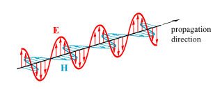
If we look for skyrmions in the cross-section of an optical beam, the electric field will itself be effectively two-dimensional and lying in the plane without a component along the propagation direction. For a skyrmion, we need a field that is three-dimensional.

However, the first 2018 demonstration⁴ of an optical skyrmion was based on the electric field using a very special experimental configuration. The trick they used was the phenomenon known as surface plasmons: on the surfaces of some metals it is possible to induce an electromagnetic surface wave that can propagate “long” (i.e. millimeter) distances along the surface without loss. These plasmons have a component of the electric field along the direction of propagation and a component perpendicular to the surface, and the field decays in amplitude away from the surface. I have crudely illustrated this below.

The 2018 researchers combined 3 pairs of counterpropagating plasmons, basically surface plasmons converging from six directions, to construct a lattice of electric field skyrmions. The plasmons provide an electric field that can point in all directions in three dimensions while the use of counterpropagating plasmons results in a field with no “out of phase” component, providing good conditions for skyrmion creation. My simulation of their results is shown below.

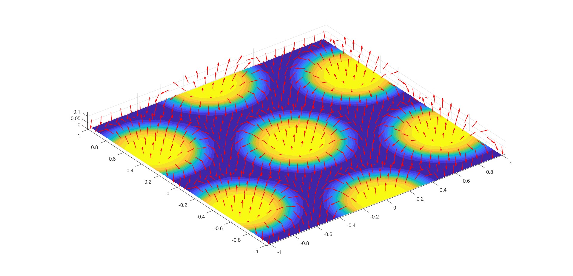
In this case you can see that we do not get a single skyrmion but instead an array of skyrmions of the same skyrmion number all arranged in a hexagonal array. This is a very common configuration that also appears in magnetism.

But surface plasmons are effectively stuck to the metal surface that they are generated on and therefore not terribly useful for desired applications like free space optical communication. To make optical skyrmions useful, one needs to be able to generate them in optical beams that can propagate long distances. Fortunately, there is a way to define a skyrmion for beams, though we need to talk about a little more optics first!

What we need is a bit of discussion of the polarization of light. In the picture of a transverse electromagnetic wave we shared above, the electric field oscillates up and down in space and time. But there are many ways that a monochromatic electric field can oscillate! At a particular point in space, the electric field can have a variety of states of polarization, as illustrated below.

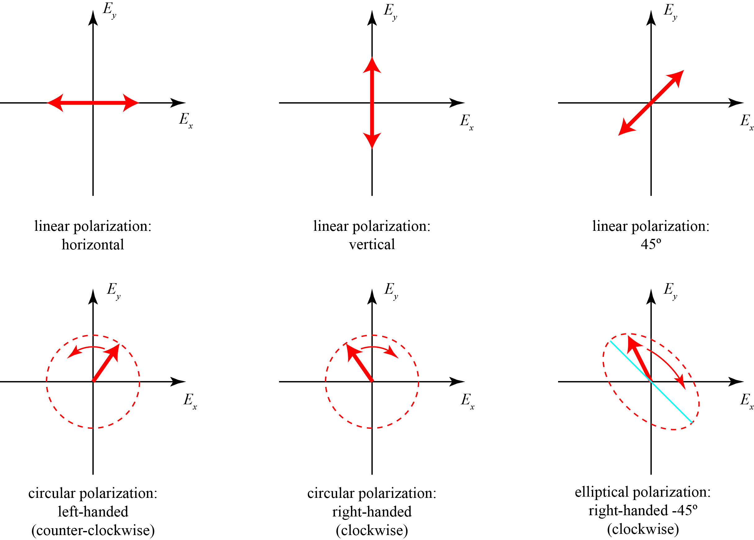
Light can be linearly polarized — oscillating side-to-side — in any direction, but it can also be circularly polarized, where the field goes in a circle. Most generally, the electric field can trace out an ellipse, in which case it is called elliptical polarization. All of these different polarization states oscillate perpendicularly to the direction the wave is going.

What is striking is that we can define a sphere, called the Poincaré sphere, where every point on the sphere represents a distinct state of polarization! This is usually illustrated as follows.

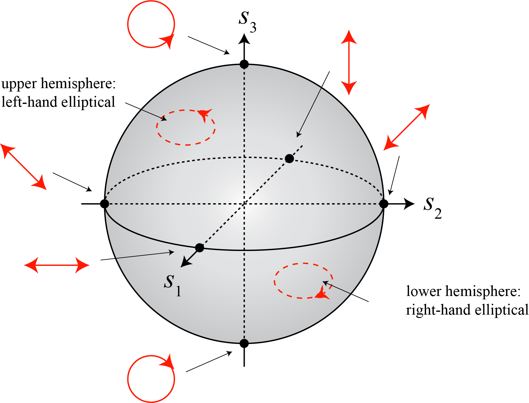
The quantities s₁, s₂, and s₃ are called the Stokes parameters and giving the Stokes parameters is equivalent to describing the position on the Poincaré sphere.

But represents a direction in a generalized space as well, and we can therefore use this as the directional quantity that defines our skyrmion. This approach was apparently first considered⁵ in 2020, and it is now the standard way to define an optical skyrmion. The Stokes parameters are easy to experimentally measure so it is in principle straightforward to measure an optical skyrmion in a beam of light.

How does one make such a Stokes-based skyrmion beam? One constructs what is known as a full Poincaré beam but taking the superposition of an ordinary Gaussian beam with left-hand circular polarization and a vortex beam with right-hand circular polarization. The result is a beam which possesses every state of polarization in its cross-section, which also in this case results in a skyrmion with skyrmion number 1. (Full Poincaré beams apparently do not always result in skyrmions, but there is a close connection.)

You’ve already seen what this skyrmion looks like, as it was the “single skyrmion” image I shared earlier!

Do optical skyrmions represent a new approach for doing optical communications? I imagine it remains to be seen, as the topic is still relatively new in optics. But hopefully, in spite of this post being long and more complicated than my usual fare, you have a little bit of an idea of what a skyrmion is now!

Postscript: I have noted that the skyrmions discussed in optics are typically called “baby skyrmions,” which raises the question: what is a regular skyrmion? To recap: a baby skyrmion is a two-dimensional field of three-dimensional directions, or a two-dimensional field of points on the surface of a normal sphere. My understanding is that a regular skyrmion is a three-dimensional field of points on the surface of a 4-dimensional hypersphere!

**********************************

1. T. H. R. Skyrme; A non-linear field theory. Proc. A 1 February 1961; 260 (1300): 127–138.
2. John Frederick Nye, Michael Victor Berry; Dislocations in wave trains. Proc. A 1 January 1974; 336 (1605): 165–190.
3. S. Mühlbauer et al. ,Skyrmion Lattice in a Chiral Magnet. Science 323, 915-919 (2009).
4. S. Tsesses et al., Optical skyrmion lattice in evanescent electromagnetic fields. Science 361, 993-996 (2018).
5. Sijia Gao, Fiona C. Speirits, Francesco Castellucci, Sonja Franke-Arnold, Stephen M. Barnett and Jörg B. Götte, Paraxial Skyrmionic Beams, Phys. Rev. A 102 (2020), 053513.